Copyright © David Boettcher 2005 - 2026 all rights reserved.
In 1658, the great English scientist Dr. Robert Hooke had the idea of using a balance spring to improve the timekeeping of watches. Because of the linear relationship that Hooke had discovered between the force applied to a spring and its extension, he thought that it would make a watch an even better timekeeper than a pendulum clock.
The balance of a watch swings backwards and forwards in rotation around a fixed axis impelled, if perfectly poised, only by its spring. A watch balance therefore does not suffer from the problem of “circular error” caused by the unidirectional pull of gravity that prevents pendulums from being isochronous.
Hooke realised that by adding to the balance a spring that obeyed his famous law, ut tensio, sic vis, “as the extension, so the force”, meaning that the tension or force generated by a spring is in proportion to the amount by which it is extended or stretched, the conditions for an isochronous harmonic oscillator would be fulfilled.
Hooke showed a pocket watch with a balance spring to Lord Brouncker, Robert Boyle and Robert Murray, seeking their sponsorship in an application for a patent on the idea. A draft patent was drawn up in 1665, but then development of balance spring watches was put on hold and the application for a patent was never submitted. Hooke was very busy at the time with many scientific investigations and, from 1666, with supervising the rebuilding of London after the Great Fire.
Nearly 20 years after Hooke had the idea, Christiaan Huygens successfully applied the spiral balance spring to watches in 1675. He announced this as an invention of his, to Hooke's great annoyance. It appears that Huygens did not conceive the idea entirely independently, but was told of Hooke's idea by Henry Oldenburg, the secretary to the Royal Society. Oldenburg’s minutes record Hooke demonstrating a spring-regulated watch to the Royal Society in June 1670, and Oldenburg is known to have corresponded with Huygens.
It was Hooke who first had the idea of applying a spring directly to the balance, but it was Huygens who, many years later, came up with the idea of using a spiral spring, something that had eluded Hooke.
With the invention of the balance spring, watches became quite good timekeepers and even at the end of the seventeenth century a verge watch could be expected to keep time to within a few minutes a day, if it was kept at a constant temperature. However, its rate would alter by around 10 or 11 seconds per day for every degree centigrade change in temperature. This effect was probably too small to be noticed by Hooke, but it was observed and documented by the brilliant and meticulous Ferdinand Berthoud.
By the early eighteenth century, when John Harrison started to constructed marine timekeepers in an attempt to meet the requirements of the Longitude Act to qualify for a reward, the effect of temperature was well known. All of Harrison's marine chronometers have devices that compensate for the effects of temperature, and they could not have achieved the accuracy that they did without them.
The story of improvement in the accuracy of balance controlled watches after Harrison had achieved the accuracy required by longitude act is very largely the story of reducing the effects of temperature on their rate.
Temperature Effects in Watches

Compensation Balance and Spring: Click to enlarge
The timekeeping of a clock is usually determined by a pendulum swinging to and fro under the effect of gravity, with a little push, called an impulse, from the escapement every time the pendulum swings through its lowest point, which is accompanied by a gentle tick. A pendulum can't be used in a watch because the watch might be held at any angle but gravity only pulls downwards, so an alternative oscillator is needed. This is provided by the balance and balance spring. The image here shows a watch balance and balance spring. The balance comprises a central bar or arm and a circular rim. The arm has an axle passing through it at right angles about which it can rotate that is called the "balance staff".
The escapement mechanism pushes the balance so that it rotates in one direction and then the other. In early watches, which didn't have balance springs, the rate at which the balance went backwards and forwards was determined solely by how hard it was pushed by the mainspring, which is why the fusee, or an alternative called a stackfreed, that equalises the torque from the mainspring was vital in such watches. Without a fusee or stackfreed the rate would change so much as the mainspring ran down that the watch would be useless as a timekeeper. Even with one, early watches without balance springs were poor timekeepers.
The addition of the balance spring transformed the timekeeping capabilities of watches by giving the balance a "natural frequency". The spring causes the balance to oscillate at this frequency, to which it returns after a disturbance. The less the balance and spring are disturbed the better the timekeeping, which is why detached escapements which only interfere with the balance over a short part of its arc, are better.
The image here shows a balance and balance spring. The balance spring is the blue spiral in the middle of the image. It is blue because it is made of high carbon steel that has been hardened and then heated until it turns blue to temper it to spring hardness. At its inner end it is attached to the balance staff by the brass collet. The inner end of the spring enters a tangential hole in the collet and is fixed in place by a pin. The outer end of the spring is fixed to the balance cock of the movement by the brass stud at its outer end.
The balance spring in the image is not a perfect spiral. This is not a fault, its outer turn is bent up above the plane of the spring and towards the centre in a Breguet overcoil. This is to allow the spring to expand and contract concentrically around the axis of the balance staff and improve isochronism.
The rim of the balance has a thin inner steel layer and a thicker outer layer of brass, and is cut through in two places near to the spoke. The two sections of the rim are bimetallic strips that bend in or out in response to temperature changes, to compensate for other temperature effects.
In a pendulum clock the principal effect of an increase in temperature is that the pendulum becomes slightly longer. In a domestic pendulum clock, the effect of this is usually negligible unless a high level of precision is required. A similar effect occurs in watches, the diameter of the balance increases with temperature. However, this is opposed by similar dimensional changes in the balance spring and the overall effect on timekeeping is small.
Ferdinand Berthoud
Ferdinand Berthoud was the first to tabulate in 1773 the effects of temperature on one his marine watches. He recorded that a temperature change from 0° to 27° Réaumur (0 to 33.75 Celsius, 32 to 92°F) caused it to lose 393 seconds in 24 hours which he apportioned as follows:
| Berthoud's observation and apportionment | |
|---|---|
| by expansion of the balance | 62 seconds |
| by loss of the spring's elastic force | 312 seconds |
| by elongation of the balance-spring | 19 seconds |
| Total loss per day | 393 seconds |
The reasoning behind Berthoud's apportioning of the individual losses is not known, and it is not entirely correct. It was accepted until 1882 when Mr T. D. Wright of the BHI, pointed out that the stiffness of a spring is proportional to its width and inversely proportional to its length, and as these two dimensions are affected in equal ratio by changes of temperature, there is no overall effect on the stiffness of the spring.
However, Berthoud's assignment of the majority of the loss to a decrease in the stiffness of the spring is correct. The overall loss of 393 seconds in 24 hours due to a change in temperature of 33.75 degrees Celsius equates to 11.6 seconds per day per °C, which is in line with other observations.
Effects of Elasticity
In a watch, a much more significant effect of increasing temperature is that the modulus of elasticity, also called Young's modulus, of the balance spring reduces. The effect of this is that the spring produces less force for a given angle of rotation. This effect is many times larger than that from the lengthening of a pendulum rod or increasing the diameter of the balance.
A watch that is carried in the pocket or worn on the wrist is kept at a fairly constant temperature by warmth from the body, which mitigates the problem to an extent, but it is usually taken off overnight and becomes cooler. However, precision time references are not normally worn and are therefore subject to all the temperature fluctuations of nature, which were more significant in a time before houses and workshops were heated.
The rate of a watch is determined by the rotational ‘moment of inertia’ of the balance and the stiffness of the balance spring. The period \(T\) is given by:
\[ T = 2\pi \sqrt \frac {I}{S} \]
where \(I\) is the moment of inertia of the balance and \(S\) is the stiffness of the balance spring. This equation gives the period of one complete oscillation of the balance or two vibrations. A vibration is half a complete oscillation, which is often used by horologists because it is the time between ticks.
The equation above can be expanded by substituting the dimensions and material properties of the balance and spring as follows:
| $$ T = 2\pi \sqrt \frac {12 m k^2 l}{t^3 E h} $$ |
m : Mass of the Balance |
With an increase in temperature, thermal expansion causes the balance to increase in diameter, which increases its rotational inertia and, all other things being equal, would cause the watch to run slower, i.e. a decrease in rate. Changes in elasticity of the material of the balance have no effect on timekeeping.
An increase in temperature causes the balance spring to expand in all directions, thickness, height and length. The increases in height and length have opposite effects on the stiffness of the spring and cancel each other out. The increase in thickness makes the spring slightly stiffer, which causes an increase in rate.
If all the terms in the equation above that do not change with temperature, π and the square root of (12 times the mass m and the ratio of length to height), are aggregated into a single constant, the period can be expressed as:
$$ T = {constant} \frac { k }{ \sqrt{t^3 E} } \space\space\space\space or \space\space\space\space T \propto \frac { k }{ \sqrt{t^3 E} } $$
This shows that as temperature changes, the period will be proportionally affected by changes in the radius of gyration of the balance, and inversely proportionally by the square root of changes in the thickness of the spring and its modulus of elasticity. An increase in the radius of gyration of the balance due to thermal expansion will increase the period, which will make the watch run slower. An increase in the thickness of the spring due to thermal expansion will decrease the period, which will make the watch run faster.
The effect on timekeeping of dimensional changes in the balance and balance spring are vastly outweighed by changes in the modulus of elasticity of a carbon steel balance spring. The modulus of elasticity of a carbon steel balance spring decreases significantly as the temperature increases, which makes the spring weaker as the temperature increases and causes a decrease in rate.
If a watch has a brass balance and carbon steel balance spring, it would lose over 10 seconds per day for a rise in temperature of just 1°C. It might be thought that a watch with a steel balance, which has nearly half the thermal expansion of a brass balance, would be better, but in fact a watch with a steel balance would lose "only" just under 10 seconds a day for the same 1°C temperature rise. The material the balance is made from has very little effect on temperature errors. The major source of error is the change in the elastic modulus of the spring.
The individual effects for both brass and steel balances are tabulated below.
| Change in rate (seconds per day) for 1°C rise in temperature | ||
|---|---|---|
| Brass balance | Steel balance | |
| Balance thermal expansion | -1.60 | -0.90 |
| Spring thermal expansion | 1.35 | 1.35 |
| Spring decrease in Young's modulus | -11.37 | -11.37 |
| Totals (- indicates loss) | -11.62 | -10.92 |
The thermal expansion of the spring and the brass balance somewhat compensate each other. The expansion of the thickness of the spring makes it stiffer and, all other things being equal, would make the watch run faster by about 1.35 seconds per day.
Thermal expansion of the brass balance increases its radius of gyration, and hence its moment of inertia, which would make the watch run slower by about 1.6 seconds per day. The two effects, increasing spring thickness and increasing balance moment of inertia, oppose and partially cancel each other. In aggregate they contribute only ¼ second per day to the overall loss of over 11 seconds.
With a steel balance the gain in rate due to the increase in stiffness of the spring is actually greater than the loss due to the increased moment of inertia of the steel balance, resulting in a gain in rate of 0.45 seconds per day, reducing the overall loss to less than 11 seconds per day.
It is the change in Young's modulus of the balance spring that contributes the remaining amount. For a brass balance, the decrease in Young's modulus with temperature contributes 98% of the loss. For a steel balance, the decrease in Young's modulus with temperature turns the small gain of 0.45 seconds per day due to the expansion of the balance spring into an overall loss of 10.92 seconds per day.
Sir George Biddell Airy, the Astronomer Royal from 1835 to 1881, showed by experiment in 1859 that a chronometer with a plain brass balance lost 6.11 seconds in 24 hours for each degree Fahrenheit increase in temperature, equivalent to 11 seconds per day per degree centigrade, which is in very close agreement with the loss of 11.62 seconds calculated above.
The bottom line is that a watch that is not compensated for temperature variations can be expected to lose or gain around 11 seconds per day for every one degree change in temperature. If such a watch was adjusted to run correctly on the watchmaker's bench at, say, 20°C, which is perhaps the same temperature at which it might spend eight hours overnight on the bedside table, and then it was strapped to your wrist at 34°C for the remaining 16 hours of the day, you could expect it to lose over a minute and a half each day.
The fact that most watches do not show such alarming changes in rate is due either to aspects of their design (compensation balance) or materials (autocompensating balance springs) that compensate for or nullify the effects of temperature changes.
Back to the top of the page.
Temperature Compensation
John Harrison was the first person to successfully apply temperature compensation to a balance controlled timekeeper, in a pocket watch made for him in 1753 by John Jefferys to Harrison's specification. This was the first watch with temperature compensation, and also the first fusee watch with maintaining power, which kept the watch going as it was being wound. Before this invention, fusee watches without maintaining power stopped as they were being wound, losing accuracy. The Jefferys watch also has Harrison's version of the verge escapement, which includes verge pallets with cycloidal backs.
All of Harrison's marine timekeepers included temperature compensation. His first marine timekeeper now called H1, which was constructed between about 1728 and 1735, and the second H2, which was begun in 1737, had gridiron type bimetallic elements similar to the gridiron pendulum Harrison had invented for his land based clocks. For H3, which was begun in 1740, Harrison created a "brass and steel thermometer curb" which was a bimetallic element made from strips of brass and steel riveted together. Because of the differential thermal expansion of brass and steel - brass expands more than steel for a given rise in temperature - as the temperature rises the bimetallic curb will bend. The free end of the curb was fitted with two pins that embraced the balance spring near to the point at which it was attached to the plate, and the bending of the curb was arranged to shorten the effective length of the spring as the temperature rose, compensating for its loss of elasticity. This was the form of temperature compensation used in the Jefferys watch.
Harrison abandoned work on H3 before it was completed, and in 1755 began work on H4, essentially a large pocket watch with a verge escapement and plain steel uncut balance quite similar in overall design to the watch made for him by John Jefferys. H4 has temperature compensation by thermometer curb as used in H3 and the Jefferys watch, maintaining power, Harrison's version of the verge escapement with diamond pallets with cycloidal backs, and a train remontoire, which was its only essential difference from the Jefferys watch.
H4 was the timekeeper that successfully passed the tests stipulated by the 1714 Act of Queen Anne "An Act for Providing a Publick Reward for such Person or Persons as shall Discover the Longitude at Sea" and which resulted in Harrison eventually being awarded the prize for "finding the longitude". There is no question that H4 could not have achieved this feat without adequate temperature compensation, but Harrison was said to be unhappy with the compensation curb because he found that the balance, balance spring, and the compensation curb itself were not all affected at the same time by changes in temperature. The swinging balance and spring would have reacted to temperature changes more quickly that the stationary and more massive compensation curb, and Harrison considered that the compensation would be improved if it was in the balance itself.
The form of temperature compensation seen in nineteenth century pocket watches and early wristwatches uses a "compensation balance" with a cut bimetallic rim, which is discussed in more detail in the next section. The compensation balance was invented by Pierre Le Roy, son of Julien Le Roy, and was improved into the bimetallic form most widely seen by John Arnold and Thomas Earnshaw. The bimetallic balance rim is made of steel with a layer of brass fused onto the outside, and it is cut so in two that the two sections of the rim can bend inwards and outwards. When the temperature increases the extra expansion of the brass compared to the steel causes the bimetallic sections to bend inward. This reduces the moment of inertia of the balance, compensating for the weakening of the spring. When the temperature falls the opposite effect occurs, the bimetallic sections to bend outwards to increase the moment of inertia and compensate for the increased stiffness of the spring.
The discovery by Dr Guillaume of the strange properties of nickel steels made it possible to make balance springs whose change in elasticity with temperature is small and controllable and which could compensate for their own expansion and that of a monometallic balance. This is discussed in the section below about on autocompensating balance springs.
Back to the top of the page.
Compensation Balance
Marine Chronometer Compensation Balance
The form of temperature compensation first seen eighteenth century marine chronometers, and later in pocket watches and early wristwatches uses a "compensation balance". This followed a principle suggested by John Harrison that rather than using a bimetallic curb to alter the effective length of the balance spring in response to changes it temperature it would be better if the compensation were in the balance itself.
In 1765, Pierre Le Roy, son of Julien Le Roy, invented a balance with mercury thermometers that achieved this. Le Roy later invented a balance with rim sections made of bimetallic strips that curled inward or outward with temperature changes. After Berthoud, Arnold, and Earnshaw adopted and perfected this design, it became the predominant form of compensation balance. Thomas Earnshaw devised the method of melting and fusing brass onto a steel core.
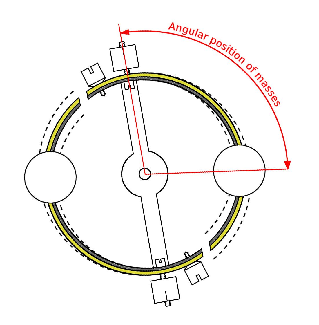
The general form of this balance is shown in the picture here. This is a sketch of the balance found in a marine chronometer, a large instrument mounted on gimbals in a cube shaped box. The balance rim is made of an inner layer of steel (coloured grey) with a layer of brass (coloured yellow) fused onto the outside. This turns the rim into a bimetallic strip and it is cut in two places near to the cross bar so that the two sections of the rim can move as shown by the dotted lines. This gives rise to the name and description of this balance as a ‘split bimetallic temperature compensation balance’, usually shortened to just ‘compensation balance’.
The operation of the balance is as follows. If the temperature increases, the brass on the outside of the rim expands more than the steel and this causes the bimetallic sections of the rim to bend inward, carrying the masses inwards towards the central axis of rotation of the balance. This reduces the moment of inertia of the balance, compensating for the weakening of the balance spring. If the temperature falls, the opposite effect occurs and the rims bend outwards, carrying the masses outward and increasing the moment of inertia of the balance, compensating for the increased stiffness of the balance spring at low temperature.
The two large masses mounted part way along the bimetallic sections were often called compensation masses, although it is their mass that contributes to the moment of inertia of the balance. The amount of compensation produced in response to a given change in temperature can be increased or decreased by sliding the masses along the bimetallic sections. The further away from the cross bar the masses are positioned, the greater the effect of the compensation.
Experiments by Kullberg in 1887 had shown that the cut bimetallic rims could be significantly affected by outward flexing. One of the balances he submitted to the Royal Observatory for testing was fitted with an "ordinary compensation balance" which had rims of thickness 0.038 inches (less than 1 millimetre) thick. The "length" of the acting laminae, the bimetallic strips, was given as 135° and the compensation masses were positioned 98° from the bar. A chronometer fitted with this balance was tested with the balance making long "arcs" of one turn and a fifth and short arcs three quarters of a turn. The arc describes the full travel of the balance from one extreme to the other so these arcs correspond to amplitudes of 216° and 135°. To someone used to working with watches these are very low amplitudes, implying a normal amplitude for a marine chronometer of 180 degrees; they were deliberately kept low to minimise outward flexing.
The mean daily rate in the short arcs was +2.6 seconds, in the long arcs it was +0.5 seconds. In the long arcs the speed of rotation was greater and the momentum of the rims and compensation masses caused the rims to flex out further than in the short arcs, increasing the radius of gyration and slowing the rate by over 2 seconds a day. This shows how important the fusee was to the performance of a chronometer with a cut bimetallic balance, because by keeping the impulse constant it kept the amplitude constant.
In "The Marine Chronometer" Commander Gould implies that the compensation masses could be at 120°, which would make the rims sections longer and the flexing effect even more prominent. In the diagram here I have shown them at 98° as per Kullberg's data.
Longines 13.34 Movement with Cut Bimetallic Compensation Balance: Click image to enlarge
The two large screws at the end of the cross bar are mean time screws, used to adjust the rate when the best temperature compensation has been established, the two small screws next to them are for very fine adjustments to the rate.
In a smaller movement such as a pocket or wristwatch there is not enough room for the large compensation masses and meantime screws, so a number of small screws distributed along the length of the bimetallic sections are used. Changes in the compensation are effected by moving some of the screws, and fine adjustments are achieved by fitting thin timing washers, or by reducing the size of some of the screw heads.
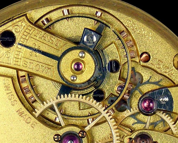
The balance shown in the photograph here is fitted to a Longines 13 ligne calibre 13.34 movement dated to 1913. It is a high grade version of the 13.34 calibre with the train jewels set in screw-set chatons, cap jewels for the escape wheel, and jewelled to the centre, giving a total of 18 jewels.
The two different metals of the balance rim, steel on the inside and brass on the outside, are visible, and it is notable that the steel is much thinner than the brass; this was to get maximum movement from the bimetallic sections. One of the two splits in the rim that allow the bimetallic sections to move is visible at the top of the photograph near to the steel stud carrier. The other split is concealed by the centre wheel. The timing screws are visible, distributed along the rims of the balance. These screws are made of gold, which was used because of its greater density compared to steel; a screw made of gold weighs more than twice as much than the same screw made of steel, and therefore is more effective in adjusting the compensation.
Uncut Compensation Balances
Watch balances are seen that look exactly like compensation balances, with brass and steel bimetallic rims, but the rim is not cut so the bimetallic strips can't curl in response to temperature changes. Sometimes the rims are cut part way through at the points near to the arms where they would be fully cut through to free the bimetallic strips.
This has long been a mystery to English watchmakers. Looking at one of these uncut balances, it occurred to me that the Swiss makers of balances might have supplied them to watchmakers in this form, which would be robust for transport, and it was the watchmaker's springers and timers who made the final cut. When a bimetallic balance rim is cut, residual stresses cause the freed bimetallic strips to spring out of shape, which then have to be bent back into being round. The process of bending the rims, poising the balance, testing the rate in different temperatures and then making further adjustments, is by far the most costly part of making a compensation balance, due to the wages of the expert springer and timer.
If I am correct, that balances were supplied by their makers uncut, the uncut balances seen in watches might be ones that, for some reason, it was decided not to spend the time and money on cutting and adjusting, but simply to fit them as they came from the balance makers.
Back to the top of the page.
Middle Temperature Error
HSN article about Middle Temperature Error.
Download article: MTE.pdf
A5639
Download spreadsheet: MTE.xlsx
S3947
I3985
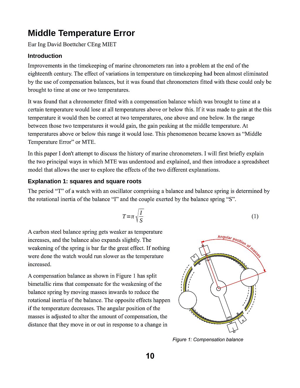
In the late eighteenth century a phenomenon was observed in marine chronometers with temperature compensation. It was found that if the device was brought to time at a certain temperature it would lose at higher and lower temperatures. This effect was not observed in watches without temperature compensation because it was dwarfed by other effects, principally the change in rate with temperature due to variation in the elasticity of the balance spring. The effect became observable in marine chronometers with compensation for this major, primary source, of temperature caused error.
To minimise the total error over the range of temperatures a marine chronometer was expected to encounter, the timing was adjusted so that it was fast at a "middle" temperature and correct at two temperatures either side of this. This gaining rate at the middle temperature was called the "middle temperature error". Because the effect only became noticeable once the primary source of error, the change in the elasticity of the balance spring with temperature, had been compensated, it was also sometimes called "secondary error".
The cause of middle temperature error has been much debated over the years since it was first observed. Qualitative explanations were advanced claiming that it was due to the effects of square or square root terms in the equation for the period of a balance. Although these explanations were logical and true, it has now been shown quantitatively that the magnitude of the error they cause is much smaller than the errors observed in practice. This is briefly outlined further down on this page and if you are not already familiar with recent discussions around middle temperature error I suggest that you read that short summary first.
This is discussed in more detail in an article published in the February 2017 edition of the Horological Science Newsletter (HSN). The article introduces a spreadsheet model that demonstrates the magnitudes of the different effects that contribute to middle temperature error. The HSN newsletter is published by NAWCC Chapter #161. The interest of Chapter #161 is the study and distribution of information about the science of horology. Chapter membership is available to members of the NAWCC. The editor of HSN, Bob Holmström, kindly agreed that my article and accompanying spreadsheet can also be downloaded from this web page.
The spreadsheet that accompanies the article allows you to interactively explore the effects of temperature on a balance and balance spring. I strongly recommend that you download and try it. You don't need to do any spreadsheet programming, it is already set up. You just alter the values of the thermal coefficients of expansion and elasticity, and charts built into the spreadsheet immediately show you the effect on timekeeping. It's really simple so give it a go, and if you have any problems just drop me an email. The spreadsheet is in Excel format. If you don't have the Microsoft Office Excel spreadsheet software, then Libre Office contains an excellent alternative that can open Excel format spreadsheets and is available absolutely free from Download Libre Office.
Spreadsheets were created to simplify and automate business models originally created with chalk and blackboards. They are a powerful tool, easy to use and incredibly useful but, like all complicated tools, if you have never been shown how to use one they can be initially daunting. I have created a very short and quick introduction into how they work to get you going. Download it from this link: Spreadsheets – A Quick Introduction (pdf). NB: Updated to Rev. 2.0 on 28 November 2017.
The spreadsheet can also be used to investigate the effects of the individual components. For example, to see the effect of thermal expansion of the balance alone, then set all the coefficients apart from the "Thermal expansion/ºC – balance:" to zero. As a check, a brass balance should show a loss of 1.64 seconds per day for a temperature increase of one degree C, a steel balance 0.95 seconds per day per degree C. The loss occurs because thermal expansion of the balance increases its rotational inertia, the difference in rates is because of the smaller thermal expansion of steel than brass.
The article and spreadsheet can be downloaded from these links: Article: MTE.pdf, Spreadsheet: MTE.xlsx.
If you have any comments or questions, please don't hesitate to contact me via my Contact Me page.
Explanations of Middle Temperature Error
An explanation for middle temperature error was developed by the Reverend George Fisher and published in The Nautical Magazine of 1842 under the name of E. J. Dent, of the chronometer makers Arnold & Dent. Fisher's name is not mentioned in Dent's article, most likely because Fisher had incurred the displeasure of the English chronometer industry by publishing a paper that suggested that the going of chronometers could be affected by magnetism in iron ships, which was wrong but potentially damaging to the chronometer industry, and Fisher probably decided to keep a low profile as a result. He continued to work on chronometers but didn't publish anything further about them.
The explanation published by Dent was based on the observation that the equation for the period of a balance controlled timepiece can be written as:
$$ T = {2 \pi} \sqrt \frac { m k^2}{S} $$
where mk2 is the moment of inertia of the balance, m being the mass and k the radius of gyration, and S represents the force or turning moment exerted by the balance spring.
Marine chronometer compensation balance
A bimetallic compensation balance alters the radius of gyration k in response to changes in temperature. The balance shown in the image illustrates how this happens. The rim of the balance is made by fusing brass onto the outside of a steel balance, and then making two cuts through the rim near to the spoke. If the temperature increases the brass expands more than the steel, which causes the bimetallic secions to curve inwards. If the temperature falls, the brass contracts more than the steel which makes the bimetallic secions curve outwards. The bimetallic secions carry masses and the radial position of these masses alters the moment of inertia of the balance. The amount of compensation can be altered by sliding the masses along the bimetallic secions. The further along the bimetallic secions that they are positioned, the greater the compensation.
If the temperature increases, the elastic force exerted by the balance spring decreases and the bimetallic sections of the balance move the compensation masses inwards to reduce the rotational inertia. The opposite happens for a fall in temperature, the bimetallic secions move the compensation masses outwards. The masses move only a very small distance and it seemed likely that they moved proportionally in response to temperature changes. Observations by Dent had suggested that the elasticity of the balance spring varied linearly with temperature, or very nearly so. In fact, Dent's data does show a non-linear effect in the spring tension, but for the purposes of explanation he assumed that it was negligible.
If the compensation was to be perfect, then from the equation above it is clear that the ratio of \(k^2\) to \(S\) must be constant. But if the masses are moved proportionally to a change in temperature, then the change in \(k\) will be linear and \(k^2\) will be a quadratic curve. Fisher realised that the curve produced by plotting \(k^2\) against temperature on a chart could only intersect with a straight line representing a linear \(S\) term at either one or, at most, two points. This is the explanation related by Commander Gould in "The Marine Chronometer" and drawn in a figure as a series of "I" curves representing the moment of inertia against a straight "S" line representing the spring term.
The Fisher / Dent explanation considers the relationship of the balance's moment of inertia to spring force within the encompassing square root sign of the equation for period. However, the encompassing square root cannot be ignored. When it is taken into account, it is evident that the period is proportional to the square root of \(k^2\); that is, the period is directly proportional to \(k\). It is clear from this that whatever is the source of the non-linearity that gives rise to middle temperature error, it is not the square in the inertia term.
An alternative way of visualising the effect is to rewrite the equation for period as:
$$ T \propto \frac { k} {\sqrt S} $$
If both k and S vary linearly with temperature, as was supposed, then a plot of k against temperature on a chart would be a straight line, but the plot of S would be a quadratic curve due to the square root. The k line could only intersect with the curve of the S term at either one or, at most, two points. This is the explanation related by A. L. Rawlings in "The Science of Clocks and Watches".
The “square root” explanation is rational, logical and correct, and it held sway as the only explanation for middle temperature error for many years. However, although the reasoning is correct, the magnitude of the middle temperature error produced by this effect is much smaller than that actually observed. There must be another, more significant, factor at work.
The shortcoming in the square root explanation was noticed by Peter Baxandall during the updating of Rawlings' classic work by the BHI, and subsequently investigated by Philip Woodward in a paper published in the Horological Journal of April 2011. Woodward showed that the middle temperature error produced by the square root effect alone was around one tenth of a second per day, only a small fraction of observed values.
The reason that the square root effect is so small is because all of the coefficients are close to unity, where unexpected things happen to square roots. Lets say we are interested in a temperature range of 30°C; that's +/- 15°C around the middle temperature. The variation in the elastic modulus is given by 1+αt, where α (alpha) is the thermoelastic coefficient and t is the temperature change. Using Rawlings' figure of -207 parts per million per °C for the thermoelastic coefficient for S (he calls it Q), at the extremes of temperature +/- 15°C the change in the stiffness of a balance spring will be 0.9969 at +15°C and 1.0031 at -15°C.
Let's just look at the second of these figures for a moment. We want the square root of 1.0031 to use on the bottom of the equation for period. Rather than reaching for a calculator, lets look at the Taylor series expansion:
\[ \sqrt{1+x} = 1 + \frac{x}{2} - \frac{x^2}{8} + \frac{x^3}{16} ... \]
Here the value of 1.0031 can be substituted for 1+x, with x = 0.0031. The third term in the series, x squared over two, will be very small and it, along with all subsequent terms, can be neglected. So when x is small like in this case, the square root of 1-x can, with a high degree of accuracy, be represented by:
\[ \sqrt{1+x} = 1 + \frac{x}{2} \]
Middle temperature error or secondary error: seconds per day.
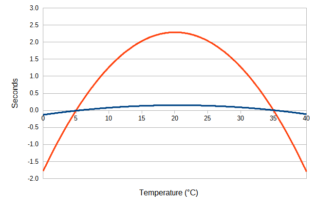
1: Blue line; square root effect alone.
2: Orange line; square root plus non-linear elasticity of balance spring.
It is immediately apparent that if the square root of the thermoelastic changes between +/- 15°C can be represented to a high degree of accuracy by the linear term on the right of the equals sign, the relationship between temperature and the stiffness of the spring is, also to a high degree of accuracy, linear. There is no doubt that the square root does cause some non-linear effect, but it is tiny. A cause for vast bulk of the middle temperature error must be sought in a different explanation.
The chart here shows the two effects on the timekeeping of a machine brought to time at 5°C and 35°C, with a middle temperature of 20°C. The blue line shows the middle temperature error that results from the square root explanation alone. It is very small, of the order of one tenth of a second per day. The orange line shows the error that results when the curvature in the temperature response of the elasticity of the balance spring is also taken into account. This results in an error of more than two seconds per day, which is in accordance with observed values of middle temperature error.
The Cause of Middle Temperature Error
In the late nineteenth century, Dr Guillaume noted that middle temperature error, which he called ‘secondary error’ or ‘Dent’s error’, is significantly reduced when a palladium alloy balance spring is used instead of a steel one. Palladium springs require slightly more overall temperature compensation than steel springs, so the reduced error is not due to smaller changes in the modulus of elasticity with temperature. It occurs because the modulus of elasticity in palladium alloys varies more linearly across the temperature range than that of steel.
The non-linear behaviour of steel springs is primarily due to their magnetic properties and crystal structure. Steel is ferromagnetic at room temperature, and changes in magnetic domain structure contribute significantly to non-linear variations in elasticity as temperature changes. Modern studies on magnetoelasticity confirm that these magnetic effects are a major source of non-linearity in the temperature–elasticity relationship for steel.
By contrast, the palladium alloys used for balance springs are non-magnetic, eliminating a major source of non-linear behaviour. In addition, palladium alloys typically have a face-centred cubic (FCC) crystal structure, which provides a more symmetrical and stable atomic arrangement than the body-centred tetragonal (BCT) or martensitic structures found in many spring steels. As a result, palladium alloy springs exhibit a more linear change in modulus of elasticity with temperature. Other effects, such as thermal expansion and alloying, play a role but have much smaller influence in comparison.
It is not clear that Guillaume ascribed any of the middle temperature error to the square root effect, he doesn't mention it in his writings. Dr Guillaume's solution to the problem of the middle temperature error can be found at The Guillaume "integral" balance.
Back to the top of the page.
The Guillaume ‘Integral’ Balance

Figure 1: Middle Temperature Error:
Click image to enlarge

Figure 2: Guillaume Integral Balance:
Click image to enlarge
The accuracy of box (marine) chronometers with steel balance springs and bimetallic compensation balances was limited by middle temperature error. Many auxiliary compensation devices were invented to counter middle temperature error, but they were delicate and difficult to adjust.
Middle temperature error arises because the modulus of elasticity of a steel balance spring does not decrease in direct proportion, or linearly, with increasing temperature, but instead follows a downward curve. A brass and steel compensation balance eliminates most of this effect by reducing its own effective diameter as the temperature increases. However, the compensation provided by a brass and steel compensation balance varies linearly, which means that it can only exactly compensate for the non-linear changes in the modulus of elasticity of a steel spring at either one middle temperature, or at two points equally distributed about the middle temperature.
To get the best overall rate, watch and chronometer makers chose the second of these, making the rate correct at two temperatures either side of the middle temperature. The chronometer or watch would then gain at temperatures between these two points, this gain being called the middle temperature error, and lose at temperatures outside.
In Figure 1, the green line labelled ‘Spring’ represents the decrease in rate caused by the reduction in stiffness of a steel balance spring with increasing temperature. The straight blue line labelled ‘Balance’ represents the increase in rate due to the inward movement of the compensation masses in response to increases in temperature. The masses are moved inwards with increasing temperature to reduce the moment of inertia of the balance to compensate for the reducing stiffness of the balance spring.
It is evident that the straight blue line of the compensation balance does not exactly mirror the green curve of the balance spring. The net effect on rate is given by the difference between the two, resulting in the curved red ‘Error’ line.
One spring evening in 1899, Dr Guillaume realised that the properties of nickel steel could be exploited to overcome middle temperature error. The steel inner layer of a bimetallic compensation balance was replaced by a nickel steel alloy called Anibal, which had the unusual property of causing the rate of compensation to increase as the temperature rose, matching the increasing loss of stiffness of the balance spring.
In Figure 2, the dark blue upward curving line shows the effect of this on the change in rate caused by the balance. The blue line of the rate due to the balance has an upwards curve that matches and mirrors the downwards curve of the green spring line, eliminating the middle temperature error and producing a flat rate over the temperature range.
To understand how Dr Guillaume created the integral balance it is useful to understand his view of how middle temperature error arises. Guillaume noted that middle temperature error, which he called ‘secondary error’ or ‘Dent’s error’, is significantly reduced when a palladium alloy balance spring is used instead of a steel one. This shows that the middle temperature error is caused by a physical characteristic of the steel balance spring.
Palladium alloy balance springs require slightly more overall temperature compensation than steel springs. This is because their modulus of elasticity change more than that of steel for a change in temperature. The reduced middle temperature error with a palladium alloy balance spring is therefore not due to a smaller change in its modulus of elasticity with temperature. The middle temperature error is reduced because the modulus of elasticity in palladium alloys varies more linearly across the temperature range than that of steel.
Compensation Balances
An ordinary compensation balance has a rim made of a layer of brass on the outside and steel on the inside, and the rim is cut in two places close to the arms.
Brass has a higher rate of thermal expansion than steel, in the ratio of about 18 to 11. As the temperature increases, the greater thermal expansion of brass than steel causes the bimetallic rim sections to curl inwards towards the axis of the balance, reducing its moment of inertia, which compensates for a decrease in stiffness of the balance spring.
The compensation provided by a brass and steel compensation balance varies linearly with temperature due to a curious coincidence in the rates of thermal expansion of brass and steel. When a piece of metal is heated or cooled by \(\pm \theta\) degrees, its length at the new temperature can be calculated using the expression,
\[ L_\theta = L_0 ( 1 + \alpha \theta + \beta \theta^2 ) \]
where \(L_0\) is the length at the initial temperature, \(\theta\) is the change in temperature and \(L_\theta\) is the length at the new temperature.
Inside the brackets, the \(\alpha\) and \(\beta\) symbols are the coefficients of thermal expansion. Frequently, only the first term with \(\alpha\) is used, but when greater accuracy is required, the second term with \(\beta\) is added. If only the first term is used, the result is that the calculated length changes in direct proportion to changes in temperature. When plotted on a graph of length versus temperature, the change in length forms a straight line, so this is referred to as linear expansion.
When the second term with \(\beta\) is added, this introduces a curve or non-linearity into the graph of change in length with temperature, because it is calculated using the square of the change in temperature. This is referred to as non-linear expansion. Ususally, the non-linear effect is small, so the plot looks like a straight line, which is why the non-linear effect is usually ignored. However, in precision horology, the non-linear effect is noticeable.
The \(\alpha\) coefficient is called the linear coefficient of thermal expansion. The \(\beta\) coefficient is called the non-linear coefficient, or the quadratic coefficient, because it involves the square of the temperature change.
Brass and steel, like most metals, have a small positive non-linear curvature in their rate of thermal expansion. This means that their rate of expansion increases as the temperature increases and their \(\beta\) non-linear or quadratic coefficient has a positive value. It is not a large effect, but it exists and can be measured.
Brass has a linear coefficient of thermal expansion of about \(18 \times 10^{-6}\)/°C whereas that of steel is about \(11 \times 10^{-6}\)/°C. The curious coincidence that causes the compensation provided by a brass and steel compensation balance to be linear is that, unlike their linear coefficients of thermal expansion, the non-linear coefficients of thermal expansion of brass and steel are virtually the same, \( 5.5 \times 10^{-9} \)/°C for brass and \(5.2 \times 10^{-9}\)/°C for steel.
Because the rates of non-linear expansion of brass and steel are virtually the same, it is effectively only the significant difference between their linear rates of thermal expansion that causes the rims to bend, so they move in or out in direct proportion to changes in temperature.
Anibal
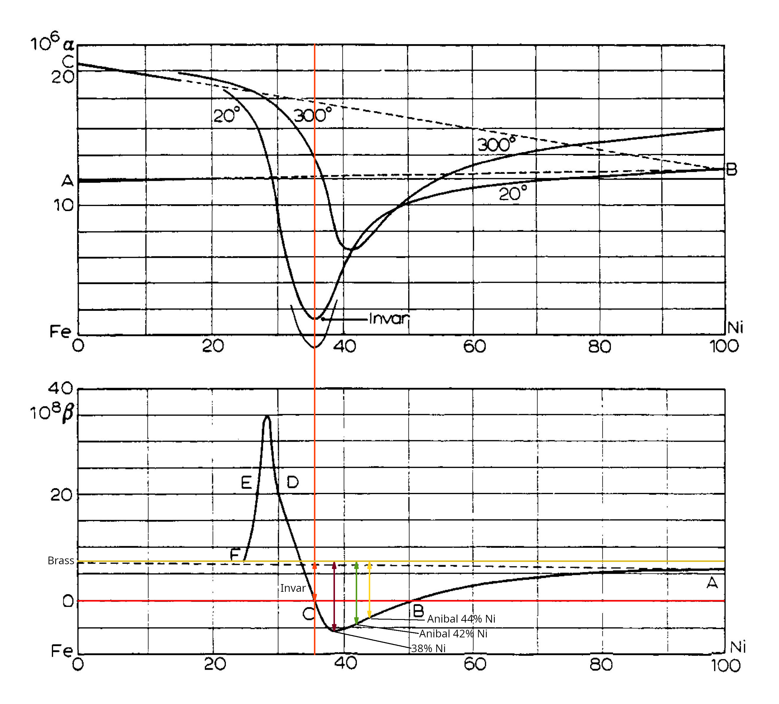
Nickel Steels alpha and beta coefficients: Click image to enlarge
Some nickel steel alloys have the unusual property that their rate of thermal expansion decreases at higher temperatures. This is characterised by a negative coefficient for the non-linear quadratic term in the thermal expansion equation.
The graph here shows the \(\alpha\) and \(\beta\) coefficients for the nickel steels. The alloy with the lowest \(\alpha\) coefficient occurs at 36% nickel and exhibits almost no change in length as its temperature is increased, for which reason it is named Invar. The lowest point of the continuous curve is at \(0.8 \times 10^{-6}\)/°C, but a short section of curve below that indicates that the coefficient can be reduced further by heat treatment and become negative, so that the material actually contracts with increases in temperature.
The red vertical line through Invar crosses the curve of the \(\beta\) coefficients at the point labelled C, exactly at zero; the zero line is highlighted in red. Between points C and B, the \(\beta\) coefficients are below zero, that is they are negative. This is very unusual, the vast majority of metals have positive \(\beta\) coefficients and expand at an increasing rate as the temperature increases.
Note that the scale of the \(\beta\) coefficients in the lower graph is different from that of the \(\alpha\) coefficients in the upper graph. The scale of the \(\alpha\) coefficients has \(10^6\) next to the \(\alpha\) at the top of the y axis. This means that the figures on the y axis have been multiplied by \(10^6\), so that the figure 20 on this scale represents \(20 \times 10^{-6}\)/°C. The y axis of the \(\beta\) coefficients has \(10^8\) next to the \(\beta\), so the 20 on this scale is actually \(20 \times 10^{-8}\)/°C. Engineers like to use powers of three, so would write this as \(2.0 \times 10^{-9}\)/°C.
The non-linear or quadratic coefficient of thermal expansion of brass is shown on the figure as the brass-coloured line at \(5.5 \times 10^{-9}\)/°C The non-linear coefficient of thermal expansion of steel lies immediately below it, where the dotted line crosses the y axis at pure iron (Fe) and 0% nickel. The non-linear rate of expansion of brass is slightly greater than that of steel, which does increase the rate of compensation of an ordinary compensation balance as the temperature increases, but the effect is small and not significant.
One evening in the spring of 1899, the idea occurred to Guillaume that if the inner steel lamina of a compensation balance was replaced by something that had a rate of non-linear thermal expansion lower than that of steel, the difference between the non-linear expansion of the brass and steel would be greater. The rate of compensation would increase as the temperature increased to more closely match the rate of decrease in the modulus of elasticity of a steel spring, and the middle temperature error would be reduced.
An obvious candidate was Invar, which has a non-linear coefficient of thermal expansion of zero, shown where the vertical red line crosses the zero axis in the lower plot. If Invar was used instead of steel, the non-linear expansion of the brass would make the rate of change of the compensation non-linear. This would reduce the middle temperature error by about 1 second in 24 hours, not enough to eliminate the full error of around 2½ seconds. This is the reason that Invar is not used in compensation balances; it would only partially correct the middle temperature error.
The degree of non-linearity in the compensation is determined by the difference between the non-linear coefficients of the two parts of the bimetallic rims, the outer brass layer which has a non-linear coefficient of \(+5.5 \times 10^{-9}\)/°C. The non-linear coefficient of Invar is zero, which in itself is unusually low, but Guillaume realised that the difference between the non-linear expansion of the brass and the inner layer would be further increased by using one of the nickel-steels that has a negative non-linear coefficient, one of the alloys between the points C and B on the graph. Referring to the graph, it is easy to see how much further away from the non-linear coefficient of thermal expansion of brass the alloys between points C and B become.
Guillaume realised that by exploiting this non-linear effect, he could alter the compensation to mirror the change in stiffness of the balance spring. Guillaume calculated that the non-linear expansion of an alloy with 44% nickel would virtually eliminate the middle temperature error. He called this alloy Anibal, from ‘acier nickel pour balanciers’ (nickel-steel for balances).
The first compensation balances with Anibal instead of steel were made by James Vaucher, a balance manufacturer in Travers. When fitted to a Nardin chronometer, the middle temperature error was reduced by about 90%. Guillaume then undertook further experimental work in conjunction with the Société des Fabriques de Spiraux Réunies to reduce the error still further. As a result of this, the nickel content of Anibal was reduced from 44% to 42%. The invention of the balance had cost Guillaume only a few calculations, but the experiments were quite expensive and consequently the results were kept secret until revealed in the early 1920s.
Looking at the plot of the \(\alpha\) and \(\beta\) coefficients for the nickel steels, the lowest point on the curve of the \(\beta\) coefficients is at around 38% nickel. Using this alloy instead of Anibal would produce too much non-linear compensation. It would cause a new middle temperature error in the opposite direction to the previous one.

Compensation Balance Non-linear Effects: Click image to enlarge
The difference between the linear coefficients of the two metals in the bimetallic rims of a compensation balance causes the rims to move in a way directly related to a change in temperature. The different metals being discussed here that could be used with brass to form a compensation balance have different linear coefficients of thermal expansion, which cause would cause different amounts of movement for a given temperature change. However, this is not important to the analysis of the non-linear effects because the compensations screws or masses can be moved along the rim to make the change in moment of inertia the same.
It is the difference between the non-linear coefficients that reduces middle temperature error, by making the compensation follow a similar curve to the changes in the modulus of elasticity of a steel spring. The effect is very small in comparison to the linear effects. The middle temperature error of a steel balance spring with a brass and steel compensation balance is about 2½ seconds per day in the middle of a 30° temperature range, whereas the change in rate due to an uncompensated steel spring over the same temperature range would be 330 seconds per day. In order to see the non-linear effects on a graph, the linear effects have to be stripped out.
The plot here called Compensation Balance Non-linear Effects shows the effects of only the non-linear coefficients of the different combinations in a bimetallic strip of brass with steel, Invar, Anibal with 44% nickel and 42% nickel, and nickel-steel with 38% nickel. One thing that is very noticeable is how flat the curve of brass with steel is almost completely flat and it is easy to see that it doesn't compensate in any way for the non-linear reduction in the modulus of elasticity of the spring. The combination of brass and Anibal with 42% nickel gives the best compensation for the non-linear changes in the stiffness of the balance spring.
The rate of thermal expansion of Anibal is smaller than than that of steel, so the difference between the linear expansion of brass and Anibal is greater than that between brass and steel. A bimetallic strip made from brass and Anibal deflects more for a given change of temperature than one made from brass and steel. In addition, to compensating for the decreasing stiffness of the balance spring as the temperature increases, a compensation balance must compensate for its own thermal expansion. In an ordinary compensation balance, the arms are steel, whereas in a Guillaume balance, they are made of Anibal. Since Anibal has a lower rate of thermal expansion than steel, the balance expands less, requiring less compensation and hence less movement of the masses.

Guillaume integral balance for a box chronometer
The Guillaume Integral balance was designed to be used with steel balance springs, the same as were used with ordinary compensation balances. This meant that in both types of balance, the compensation masses had to move essentially the same distances, although the masses in the Guillaume balance moved with the non-linearity needed to eliminate secondary error. Because the deflection of the bimetallic sections of the Guillaume balance was greater for the same temperature change, a shorter length of rim produced the necessary movement of the masses. Essentially the compensation masses of the Guillaume balance could be placed closer to the root of the strip where it is attached to the arm.
To produce the necessary movement of the compensation masses, an ordinary brass and steel compensation balance had to have long thin bimetallic rim sections. Kullberg had shown in 1887 that these were affected by outward flexing of the rims due to centrifugal force as the balance oscillated. One of the balances he submitted to the Royal Observatory for testing was an ordinary compensation balance which had rims of thickness 0.038 inches (less than 1 millimetre) thick. The length of the acting laminae, the bimetallic strips, was given as 135° and the compensation masses were positioned 98° from the bar. With such long thin bimetallic sections it is hardly surprising that the ordinary compensation balance would be significantly affected by outward flexing of the rims.
The Guillaume compensation balance produced the required movement of the masses with much shorter bimetallic sections, which were also less susceptible to outward flexing of the rims.
In addition to compensating for the reducing stiffness of a steel balance spring with increasing temperature, a compensation balance must also compensate for the radial expansion of its own arms. Anibal has a lower expansion rate than steel, which reduces the expansion of the arms, further reducing the distance that the masses on the rims need to move in or out in response to changes in temperature.
Identifying Guillaume Balances
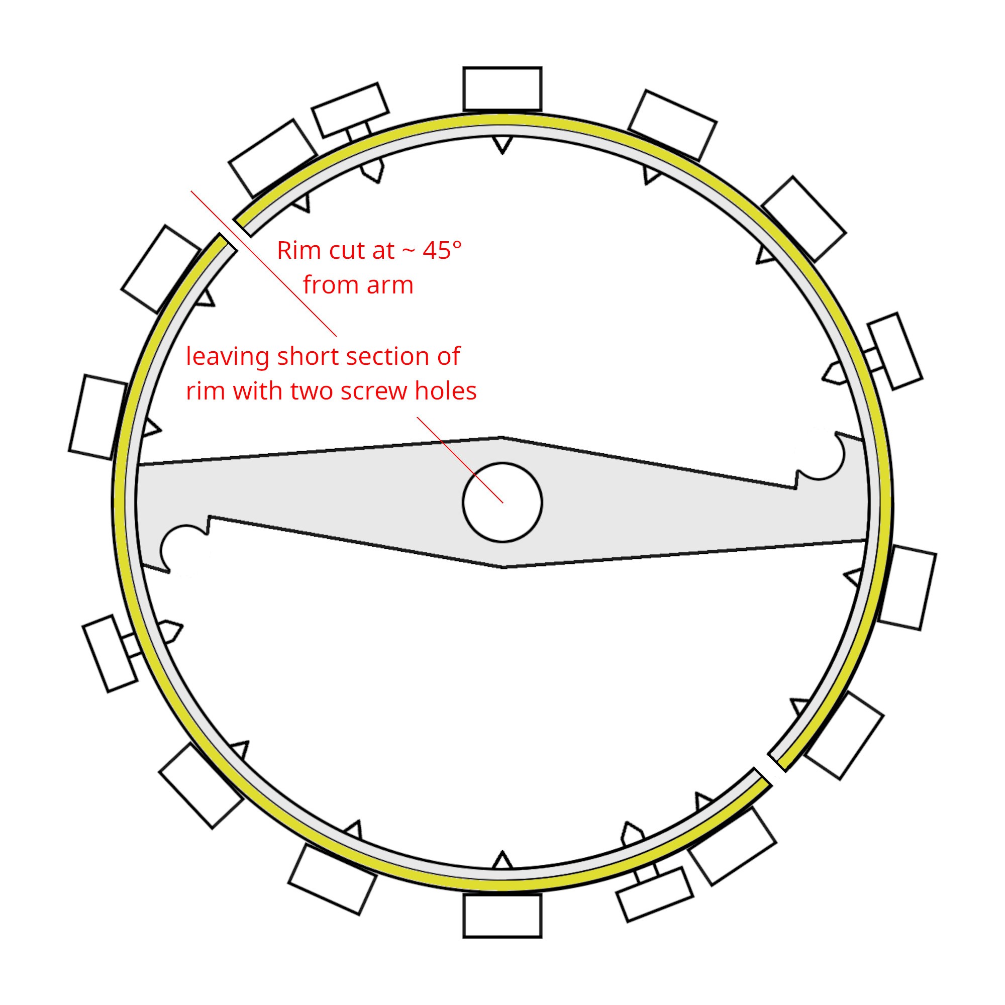
Drawing of a Guillaume watch balance:
Click image to enlarge
The extra movement of the rim sections allowed the rim of balances for box (marine) chronometers to be cut at 90° to the bar to make four short bimetallic sections, and four smaller compensation masses used. The distance these had to be moved in and out to provide the compensation was essentially the same as in the ordinary compensation balance, but instead of being positioned 100° to 120° along the rim sections, the extra movement of the rims allowed the to be at about 45°.
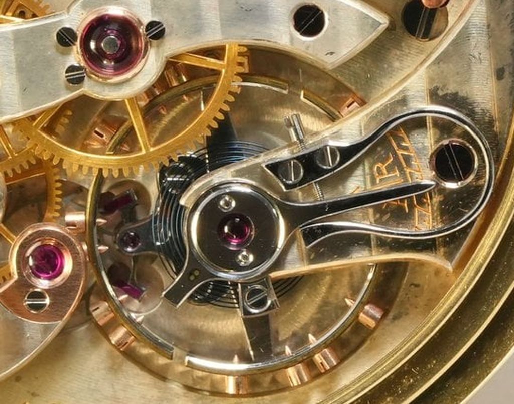
Guillaume watch balance:
Click image to enlarge
The drawing of a Guillaume compensation balance shown in the section above can be compared to the drawing of an ordinary marine chronometer compensation balance in the section about the Compensation Balance.
Guillaume balances for watches are different from those for larger box chronometers. The photo here shows a Guillaume balance in a pocket watch.
The balance is identified by the short sections of bimetallic rim next to the arms with holes for two screws. Ordinary compensation balances do not have these; the rim is cut closer to the arms.
Making Guillaume Balances
Anibal was alloyed and cast at the Imphy steelworks and supplied to balance manufacturers in Switzerland. Discs of Anibal were made from the raw material. A ring of brass was placed on the disc, with a fluz between the two. They were then heated in a furnace until the brass melted and fused onto the outer circumference of the Anibal disc.
After fusing the brass ring to the Anibal disc, the brass was in a relatively soft state, so after cleaning up it was compressed by hammering. This was a skilled task and could not be completely consistent, so later the brass was compressed by rolling between three ball races.
The outer surface of the disc was then machined to the final dimensions and the inner part cut away to form the inner Anibal rim and the arms.
Performance of Guillaume Balances
After the introduction in 1877 by Charles-Auguste Paillard of a palladium alloy suitable for balance springs, many leading English chronometer makers, after some initial resistance, adopted palladium alloy balance springs. Palladium alloy has two advantages over steel: it does not rust, and its modulus of elasticity varies more linearly with temperature. This more linear variation in the modulus of elasticity significantly reduced the middle temperature error when used with ordinary compensation balances. Britten observed that ‘The fifth chronometer on the 1883 Greenwich trial was fitted with a palladium spring and an ordinary compensation balance without auxiliary. No chronometer maker would expect such a result with a steel spring.’
The Guillaume balance was invented in 1899 and was not available commercially in time for the Neuchâtel chronometer competition in 1901. However, in the following year, 13 pocket chronometers fitted with Guillaume balances were entered. The report of the competition in the Journal suisse d’horlogerie states that these showed a variation of ±0.044 seconds per degree, a proportionality deviation of ±0.35 seconds, and a return to normal operation after thermal testing of ±0.50 seconds.
The following table summarises the results from the same competition for 21 box (marine) chronometers fitted with Guillaume balances and steel balance springs against 9 box chronometers with palladium alloy balance springs and ordinary compensation balances, and 144 chronometers with steel balance springs and ordinary compensation balances.
| Variation per 1°C ± s | Proportionality deviation ± s | Resumption of rate after thermal test ± s | Given by | |
|---|---|---|---|---|
| Guillaume balance, steel balance spring | 0.040 | 0.33 | 0.42 | 21 chronometers |
| Palladium alloy spring, ordinary compensation balance | 0.041 | 1.46 | 1.35 | 9 chronometers |
| Ordinary compensation balance, steel spring | 0.071 | 1.63 | 0.94 | 144 chronometers |
In this table:
- Variation per 1°C is the average rate variation with temperature.
- Proportionality deviation is the middle temperature error — the departure from perfectly linear compensation across the temperature range.
- Resumption of rate after thermal test measures how well timekeeping returned to normal after temperature changes.
Although the variation per degree was almost identical for palladium springs and Guillaume balances, the proportionality deviation (middle temperature error) and recovery after temperature changes were significantly better in chronometers fitted with Guillaume balances and steel springs. These results explain why continental chronometer makers quickly adopted the Guillaume balance while abandoning palladium springs, despite their earlier promise.
These results show that a steel balance spring combined with a Guillaume balance produces superior timekeeping. Although palladium alloy springs used with traditional compensation balances reduced the middle temperature error compared to steel springs, the Guillaume balance compensated the non-linear elasticity of steel springs more effectively. Steel springs had lower internal friction than palladium alloy ones, were less prone to sagging under their own weight, were easier to form accurately, and were well supported by established manufacturing techniques. The combination of a steel spring and Guillaume balance delivered better temperature compensation, better recovery after temperature changes, and superior long-term stability compared with palladium springs used with ordinary compensation balances.
The English agent for Guillaume balances, which were often incorrectly called “Invar balances”, charged 45 shillings (£2 5s) for a Guillaume balance for a marine chronometer. On top of the resistance of the English watch industry to continental inventions, this was a very high price, and few English chronometers used Guillaume balances.