Re-Identification vs Anonymization Strength

Code: github.com/mpcsb/reidentification

(I had a draft of this experiment sitting around for a while. Essentially a private exploration of privacy and utility)

The question

I generated a small synthetic dataset, anonymized its identifying attributes at increasing values of k, and tried to link the anonymized records back to the originals.

The aim was not to prove that k-anonymity is sufficient. It was to observe how re-identification risk and data resolution move as anonymization becomes more aggressive. In particular, I wanted to see whether the two changed at the same rate, and whether every attribute paid the same utility cost.

Setup

The dataset contains 2000 synthetic individuals and four fields:

I varied k from 1 to 20. A dataset is k-anonymous with respect to these quasi-identifiers when every released combination of age, ZIP3 and sex describes at least k records. To reach that condition, the routine groups or suppresses values until small groups disappear.

There were three main controls. Ages could be placed in bins from one to ten years wide; ages above a threshold could be top-coded, such as 75+; and ZIP3 values below a frequency threshold could be replaced with Other. I ran combinations of these settings because k is only part of the story. Two releases with the same k can expose quite different amounts of detail depending on how their groups were formed.

The simulated attacker knows a person’s exact age, sex and ZIP3, but does not know their glucose measurement. That knowledge is limited, although the matching procedure itself is fairly strong. Rather than matching each row greedily, I used the linear sum assignment solver in Google OR-Tools to find a globally consistent, one-to-one assignment between the anonymized and original datasets.

For an anonymized record (a_i) and an original record (o_j), the matching cost was:

[ c(i,j) = d_{age}(a_i,o_j) + d_{zip}(a_i,o_j) + d_{sex}(a_i,o_j) ]

An original age inside the released age range receives no age penalty; an age outside it receives a larger one. ZIP and sex contribute their own penalties when they do not fit the released values. The solver minimizes the sum of these costs while allowing each original record to be used at most once. This matters because a plausible match for one row can change the best assignment for many other rows.

I measured success with Hit@1: the fraction of anonymized rows assigned to their true original record. A Hit@1 of 0.5 means that the first and only guess was correct for half of the rows.

How quickly re-identification falls

The heatmaps show Hit@1 across values of k and two of the generalization controls. The first varies the age-bin width without rare-ZIP suppression. The second keeps one-year age bins and varies the threshold used to collapse rare ZIP3 values.

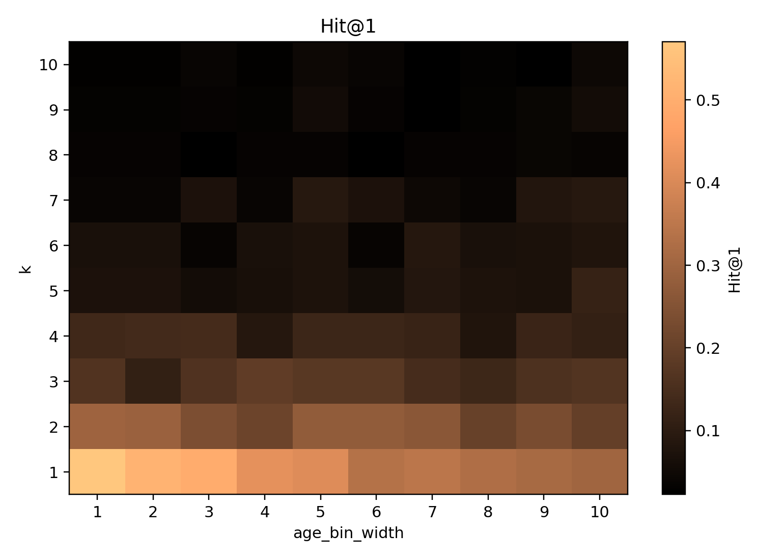
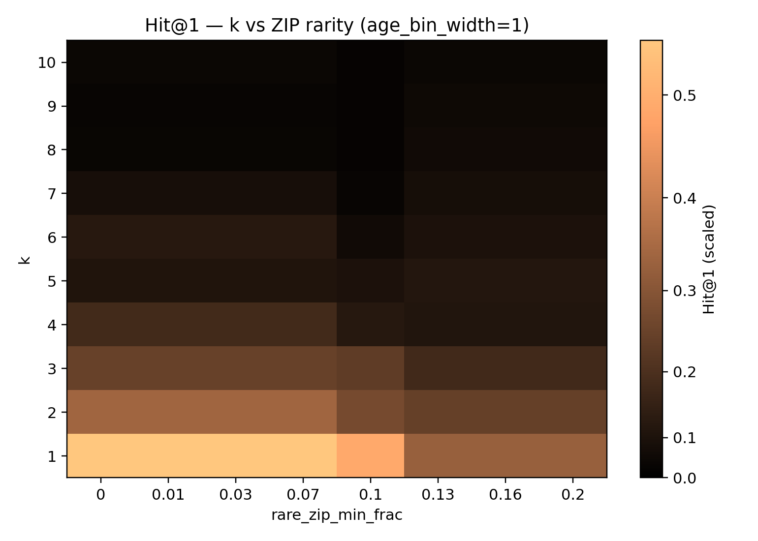
The first useful result appears at k=1. Hit@1 reaches only a little over 0.5 in the least generalized configurations, even though there is no deliberate requirement to place records into larger anonymity groups. Age, sex and ZIP3 are not unique keys: several people can share the same combination. Once that happens, the attacker cannot distinguish all of them using these attributes alone. Duplicate quasi-identifiers therefore set a ceiling on linkage success before stronger anonymization begins.

Increasing k lowers Hit@1 across the tested settings. Much of the reduction happens in the first few steps: the difference between k=1 and the low-to-moderate values is much larger than the differences among the highest values shown. By k=10, Hit@1 is low throughout these configurations.

The horizontal differences are also important. Wider age bins reduce linkage success even when k is fixed, and collapsing rare ZIP3 values changes the result again. It would be misleading to attribute every change in the heatmaps to k alone. The particular generalization rules determine what evidence remains available to the attacker.

I have not calculated a random-assignment baseline here, so “low” is the useful description for the later Hit@1 values—not “random chance.”

What the anonymization changed

I tracked utility separately for ZIP3, age and glucose. This is deliberately simpler than testing a downstream model, but it reveals which parts of the release were actually changed.

ZIP utility compares the original and released ZIP3 distributions using (1 - \frac{1}{2}L_1), where 1 would mean that their category shares are identical. It declines from about 0.77 at k=1 to about 0.73 at k=20.

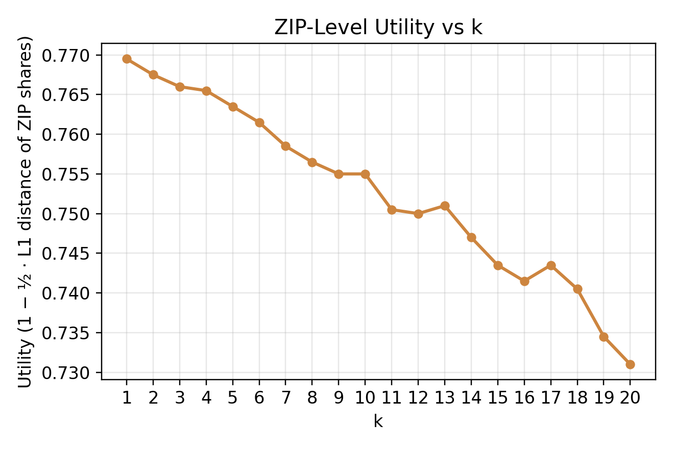
This is a gradual, measurable loss rather than a collapse. It means that suppressing rare regions changes the overall ZIP composition, but this metric alone does not support a claim that a particular percentage of geographic granularity has disappeared. It measures similarity between distributions, not the practical value of the field for every possible analysis.

Age follows a different pattern. The released mean is already about two years below the original at k=1. As k rises, the drift grows to roughly three years.

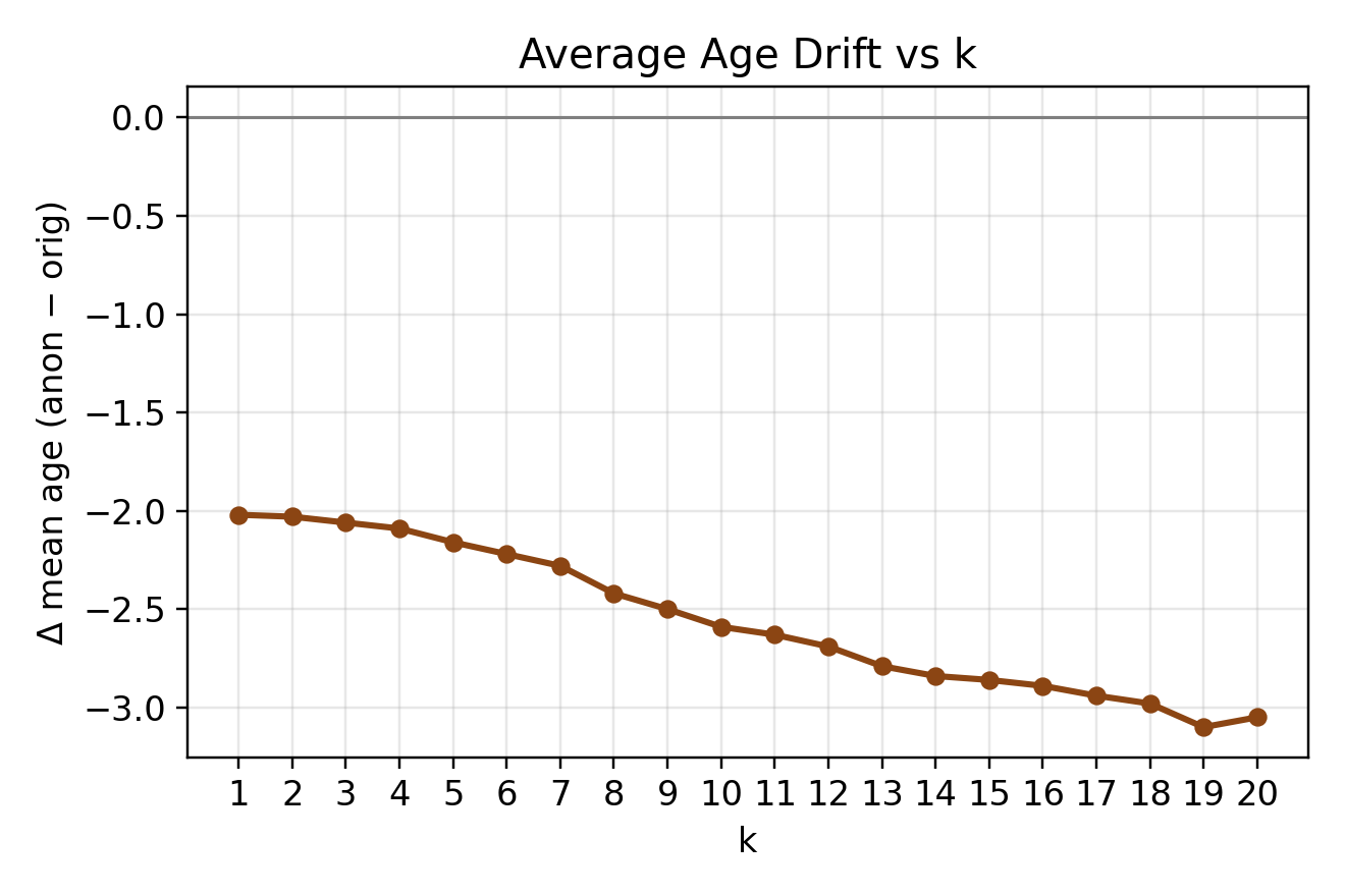
The distinction between those two amounts matters. Moving from low to high k adds around one further year of drift; it does not create the whole three-year difference. The initial offset appears to come from the baseline representation and generalization procedure, including binning and top-coding.

Glucose, meanwhile, stays essentially unchanged. The routine carries it through without transforming it because it is neither a quasi-identifier nor part of the matching cost. This does not establish that the anonymized data would remain useful for every glucose analysis—relationships with generalized age or location might still matter—but it does confirm that the marginal glucose values themselves were preserved.

Taken together, these measurements are more informative than a single utility score. ZIP composition shifts gradually, mean age has a baseline offset followed by additional drift, and glucose is left alone. Utility loss depends on the attribute, the transformation applied to it, and the analysis someone wants to perform later.

Risk and utility together

The next plots put Hit@1 and utility on the same axes. They compare selected age-bin widths and rare-ZIP thresholds, with each point labelled by k. I think of these as trade-off curves rather than strict Pareto frontiers: the figures include tested configurations, but I have not removed every dominated point or established that the curves contain all efficient choices.

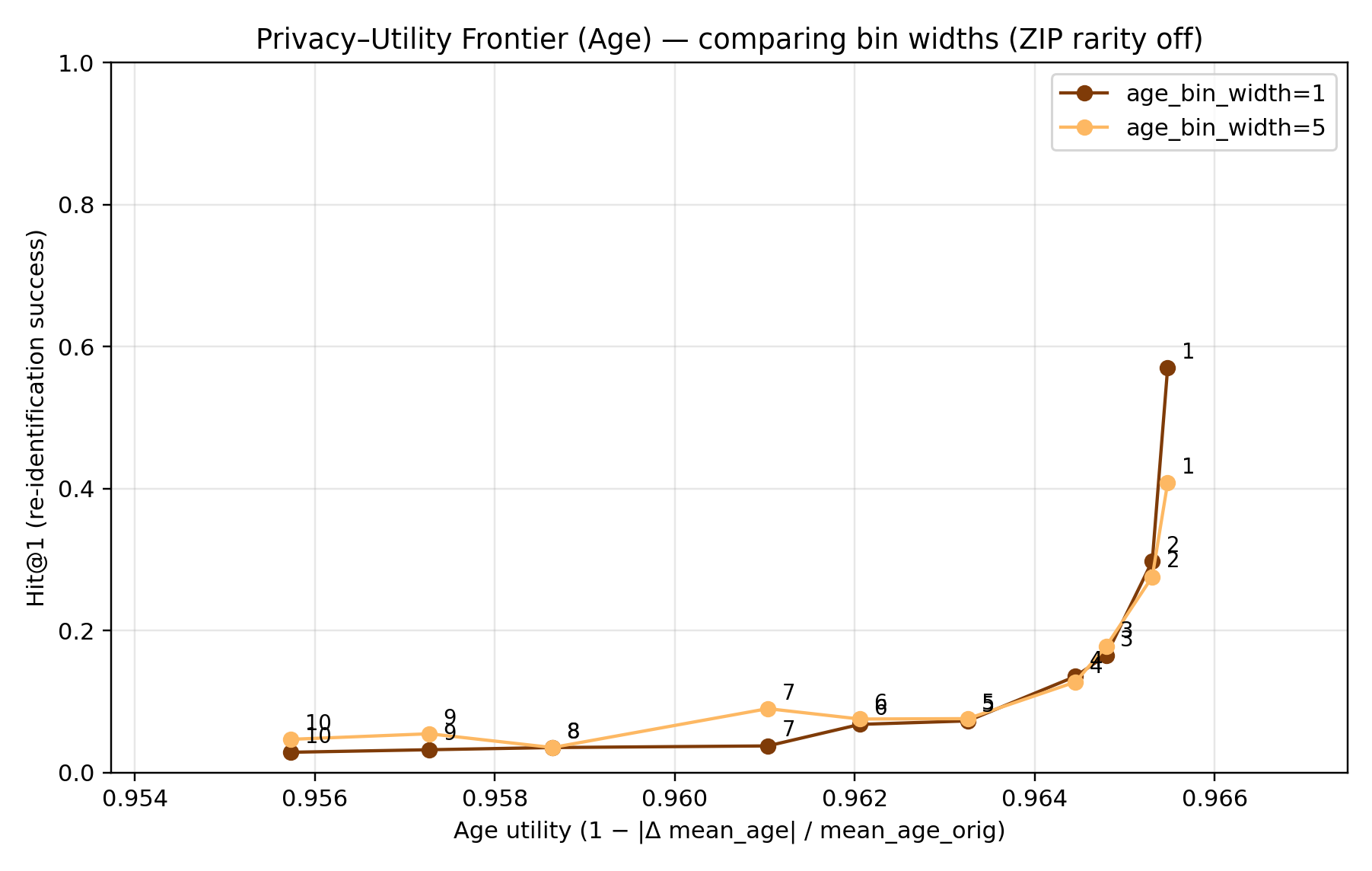
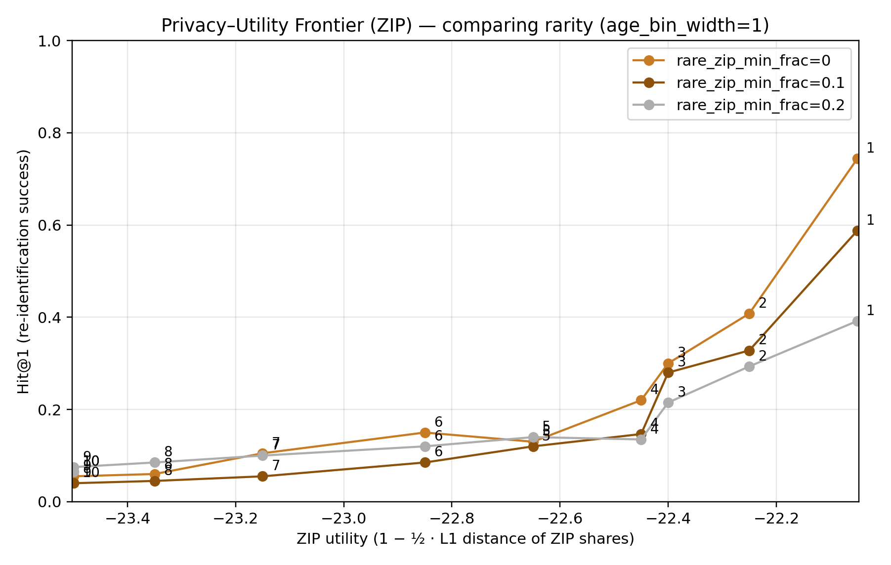
In this simulation, the first increases in k reduce linkage success more quickly than they damage these utility measures. Later increases still reduce risk, but the gains become smaller while detail continues to change. The exact path also depends on the generalization setting: changing the age-bin width or ZIP threshold can move a configuration even when k stays the same.

There is no universal sweet spot in these plots. An acceptable release for estimating an overall glucose distribution may not be acceptable for studying small geographic groups, and neither utility metric says how damaging a successful match would be. Choosing an operating point requires a concrete use for the data and a threat model, not only a preferred value of k.

Limitations and final remarks

This is a controlled simulation with one synthetic population, one anonymization routine and one attacker model. The attacker knows only age, sex and ZIP3. Given those attributes, however, the attack is not especially basic: global one-to-one optimization is stronger than independently choosing the nearest row. An attacker with extra clues, access to another leak, or a probabilistic linkage model could obtain different results. An attacker with less accurate background information could do worse.

The utility side is narrow as well. Distributional ZIP similarity and mean-age drift are useful diagnostics, but they are not substitutes for evaluating the analyses the released data is meant to support. Glucose remaining numerically unchanged is also not a guarantee that every relationship involving glucose survives generalization.

The main observations I would keep from the experiment are:

• Duplicate quasi-identifiers limit re-identification even at k=1.
• Most of the reduction in Hit@1 occurs at low-to-moderate k in this setup.
• The attacker’s knowledge is limited, but the assignment method uses the whole dataset jointly.
• Age, ZIP3 and glucose lose utility in different ways because they are transformed differently.

For this dataset, increasing k made correct linkage less common, with the largest changes arriving early. What disappeared from the data was less uniform: ZIP composition moved gradually, age drifted a little further from an existing baseline offset, and glucose values stayed intact. That conditional result is more useful than a general claim that higher k either solves re-identification or destroys the dataset.