Working at Polar Signals on the Continuous Profiling storage that is based on pprof, I had to learn more about the internals of pprof. Rather than working my way through this all alone let's take a deep dive together and see how things fit together to make the profiles we often use.
We will begin with Go structs and see how we end up with a flame graph representation of the example data we'll use.
The Profile Go struct
The fundamental building block is the profile.Profile Go struct:
type Profile struct {
SampleType []*ValueType
DefaultSampleType string
Sample []*Sample
Mapping []*Mapping
Location []*Location
Function []*Function
Comments []string
DropFrames string
KeepFrames string
TimeNanos int64
DurationNanos int64
PeriodType *ValueType
Period int64
}
Note: This struct is not the same that's used by proto which also takes care of serializing strings into the string table. That's a topic for another post.
Don't worry what all of these are just yet, as we are going to concentrate on the most important fields one step at a time to build a simple profile.
For now, let's create a test (by saving the source code as `profile_test.go`) that writes an empty profile to disk:
package profile_test
import (
"os"
"testing"
"github.com/google/pprof/profile"
)
func TestProfile(t *testing.T) {
p := profile.Profile{}
f, err := os.Create("profile.pb.gz")
if err != nil {
t.Fatal(err)
}
if err := p.Write(f); err != nil {
t.Fatal(err)
}
}
We can run the test by executing the `go test ./profile_test.go` command in our terminal.
Now next to that file you should see a file called `profile.pb.gz`. This file is just like the files you usually get from the pprof endpoints of your application, someone sends you for debugging or that people share on share.polarsignals.com for interactive debugging with others.
Currently, the profile has no samples and thus won't be able to be visualized:
Adding our first Sample with Function and Location
Now, to actually add some data to the pprof profile let's think of a simple function that we imagine to be profiling.
We want to see how many allocations that function has had since the process started. Therefore we chose the `allocs_space` profile type.
package main
import (
"os"
"testing"
"github.com/google/pprof/profile"
)
func TestProfile(t *testing.T) {
p := profile.Profile{}
+
+
+ p.SampleType = []*profile.ValueType{{
+ Type: "alloc_space",
+ Unit: "bytes",
+ }}
f, err := os.Create("profile.pb.gz")
if err != nil {
t.Fatal(err)
}
if err := p.Write(f); err != nil {
t.Fatal(err)
}
}
Let's add a Sample (a measurement) of a function that we say had allocated 128 bytes:
package main
import (
"os"
"testing"
"github.com/google/pprof/profile"
)
func TestProfile(t *testing.T) {
p := profile.Profile{}
p.SampleType = []*profile.ValueType{{
Type: "alloc_space",
Unit: "bytes",
}}
+ p.Sample = []*profile.Sample{{
+ Location: nil,
+ Value: []int64{128},
+
+ }}
f, err := os.Create("profile.pb.gz")
if err != nil {
t.Fatal(err)
}
if err := p.Write(f); err != nil {
t.Fatal(err)
}
}
The visualization won't show anything yet, as we don't have any Location given, but on of the most important data points has been filled.
The `Value` of a Sample is a slice `[]int64` because, if we were to have more sample types than just _alloc_space_, for example, _in_use_, we would add the second Value as `[]int64{128, 100}`. That means that the order of `SampleType` dictates the order of Values too.
Next, let's add a Location that describes where in the memory the sample was recorded:
package main
import (
"os"
"testing"
"github.com/google/pprof/profile"
)
func TestProfile2(t *testing.T) {
p := profile.Profile{}
p.SampleType = []*profile.ValueType{{
Type: "alloc_space",
Unit: "bytes",
}}
+
+ p.Location = []*profile.Location{{
+ ID: 1,
+ Address: 123456789,
+ }}
p.Sample = []*profile.Sample{{
- Location: nil,
+ Location: []*profile.Location{p.Location[0]},
Value: []int64{128},
}}
f, err := os.Create("profile.pb.gz")
if err != nil {
t.Fatal(err)
}
if err := p.Write(f); err != nil {
t.Fatal(err)
}
}
As you can see we have now added one Location with the memory address `123456789`. Our sample from before now references that Location.
Visualizing the profile, by running `go test profile_test.go` and then `go tool pprof -http=:8080 profile.pb.gz`, now shows the following graph:
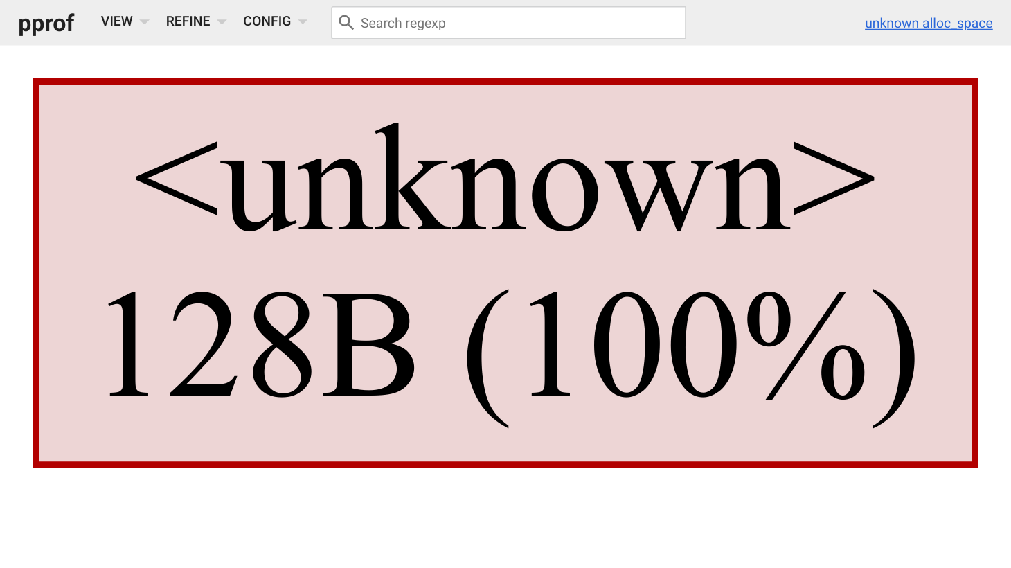
Exciting! We can see that something has used 128B (bytes)! 🎉
Because the `Mapping` is unknown for the `Location` it shows <unknown>. Adding a `Mapping` would already show the `Mapping` file name. For keeping this post shorter we'll skip this step.
Let's fix the naming next!
package main
import (
"os"
"testing"
"github.com/google/pprof/profile"
)
func TestProfile(t *testing.T) {
p := profile.Profile{}
p.SampleType = []*profile.ValueType{{
Type: "alloc_space",
Unit: "bytes",
}}
+
+ p.Function = []*profile.Function{{
+ ID: 1,
+ Name: "simpleFunction",
+ SystemName: "simpleFunction",
+ Filename: "main.go",
+ StartLine: 0,
+ }}
p.Location = []*profile.Location{{
ID: 1,
Address: 123456789,
+ Line: []profile.Line{{
+ Function: p.Function[0],
+ Line: 42,
+ }},
}}
p.Sample = []*profile.Sample{{
Location: []*profile.Location{p.Location[0]},
Value: []int64{128},
}}
f, err := os.Create("profile.pb.gz")
if err != nil {
t.Fatal(err)
}
if err := p.Write(f); err != nil {
t.Fatal(err)
}
}
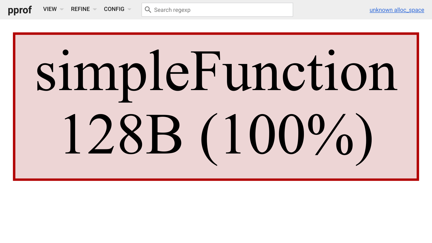
Running `go test profile_test.go` once again and then opening the profile with `go tool pprof -http=:8080 profile.pb.gz ` shows us that indeed we've now added the needed metadata to the sample. 😎
A slightly more complex sample
So far the profile is far from what you'd actually see in reality therefore let's create a somewhat more complicated sample.
package main
import (
"os"
"testing"
"github.com/google/pprof/profile"
)
func TestProfile(t *testing.T) {
p := profile.Profile{}
p.SampleType = []*profile.ValueType{{
Type: "alloc_space",
Unit: "bytes",
}}
p.Function = []*profile.Function{{
ID: 1,
Name: "simpleFunction",
SystemName: "simpleFunction",
Filename: "main.go",
StartLine: 0,
+ }, {
+ ID: 2,
+ Name: "badFunction",
+ SystemName: "badFunction",
+ Filename: "storage.go",
+ StartLine: 22,
+ }, {
+ ID: 3,
+ Name: "badSubFunction",
+ SystemName: "badSubFunction",
+ Filename: "storage.go",
+ StartLine: 42,
}}
p.Location = []*profile.Location{{
ID: 1,
Address: 123456789,
Line: []profile.Line{{
Function: p.Function[0],
Line: 42,
}},
+ }, {
+ ID: 2,
+ Address: 234567890,
+ Line: []profile.Line{{
+ Function: p.Function[1],
+ Line: 22,
+ }},
+ }, {
+ ID: 3,
+ Address: 234567891,
+ Line: []profile.Line{{
+ Function: p.Function[2],
+ Line: 42,
+ }},
}}
p.Sample = []*profile.Sample{{
Location: []*profile.Location{p.Location[0]},
Value: []int64{128},
+ }, {
+ Location: []*profile.Location{p.Location[2], p.Location[1]},
+ Value: []int64{128 * 4},
+
}}
f, err := os.Create("profile.pb.gz")
if err != nil {
t.Fatal(err)
}
if err := p.Write(f); err != nil {
t.Fatal(err)
}
}
As you can see we've added two new Functions, two new Locations, and then one new Sample.
The most important difference now is that the Location field of the Sample contains multiple Locations.
The order of these Locations is what makes up the underlying stack trace. In this example, it means that the `Location[1]` (our badFunction) was a function that called another function at `Location[2]` (our badSubFunction). Note, that somewhat counter-intuitively the first `Location` is the leaf and the last `Location` is the root of the stack trace. Each profile may contain many of these stack traces that make up the profiles as you normally see them.
Let's see how it looks visualized by running `go test profile_test.go` and `go tool pprof -http=:8080 profile.pb.gz`.
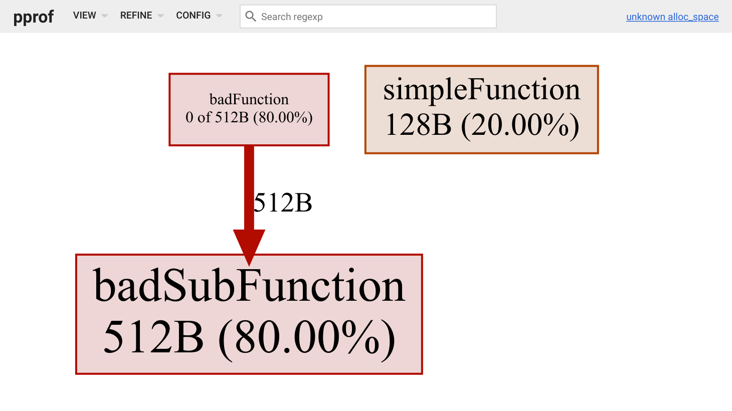
Perfect, just as we've hoped for we can now see visualized how the badFunction calls the badSubFunction that allocates four times as much as the simpleFunction from the previous example.
Conclusion
At first, the Go struct might not intuitively make sense. Maybe the `Functions` field makes sense, but working out way step by step from an empty profile to something the reassembles what we usually look at made understanding easier.
We started out by creating a single Sample that on its own was not that helpful yet. Therefore we created a Location next and referenced it from our sample - our first visualized graph still showing `<unknown>` though. We added a Function that we can reference from the Locations Line so that we get some actual function name. Our first full graph was done!
To make things a bit more realistic we've added multiple Samples, Locations, and Functions next to see how stack traces are represented. Exciting! 🎉
Going forward, you shouldn't be all too afraid when opening your editor and working with the in-memory representation of a profile.
If you would like to discuss this post, feel free to join our Discord community server!