Artificial intelligence models development for profitability factor prediction in concentrated solar power with dual backup systems

Overview

Most developed nations have plans and goals to soon reduce reliance on fossil fuels in generating power and employ alternative and renewable resources like solar and wind energy, in addition to the environmental issues connected with a nonstop rise in global energy consumption¹. In this context, the global vision for 2050 will adopt a net-emission system, which promotes enhancing the capacity of renewable energy technologies to achieve the ultimate goal of energy decarbonization². Spain shut down seven coal power plants in the past three years, reaching nearly − 40.4% in the installed capacity³. A higher portion of variable renewable energy (VRE) can lead to the following two critical issues: (i) the national power grid will be unstable in production, and (ii) more backup production technologies and energy storage resources are needed^4,5. Efforts have been made to address the previous concerns by concentrating more on dispatchable renewable energy (DRE) infrastructures, such as CSP plants^6,7. In particular, the primary energy source of CSP plants is sunlight (which is abundant but intermittent). It can be hybridized with multiple backup systems such as (molten salts, phase change materials (PCM)) and (agricultural waste, wood chips) to enhance the reliability and efficiency of solar power generation⁸.

Combining CSP plants with two backup systems, such as TES (e.g., molten salts, phase-change materials) and organic materials (e.g., agricultural waste, wood chips), will extend the operational hours by utilizing stored energy when solar input is inadequate and enhance the reliability by providing a renewable and dispatchable backup energy^9,10. The CSP plants can be installed according to two critical considerations: the availability of direct normal irradiation (DNI) (which is abundant but intermittent) and the availability of combustion or biochemical processes^11,12. The hybridized CSP plants enhanced dispatch ability and flexibility in proportion to their contributions, resulting in a stable power supply with reduced solar resource fluctuation¹¹. Furthermore, hybridized CSP facilities offer advantages over standalone CSP plants. For example, merging infrastructure and equipment (such as the power block) reduces direct expenditure on capital^13,14. Additionally, hybridized CSP plants require less feedstock than conventional biomass plants, reducing storage costs¹⁵.

Literature review on hybridized CSP plants

In 1980, the first attempt to integrate CSP with biomass (waste materials) as a backup system, using dish systems was implemented¹⁶. Nevertheless, the initial commercial Borges CSP-biomass hybrid facility situated near Lleida, 150 km west of Barcelona, Spain, in 2012 experienced an additional 25-year delay for unspecified reasons¹⁷. The hybrid CSP-biomass facility in Borges generates electricity under a power purchase agreement (PPA) at a rate of $0.309 per kWh, with a net installed capacity of 22.5 MW_e. After that, two new hybridized CSP-biomass stations were established in southern Italy (2014) and Denmark (2019). The Falck CSP-biomass facility in Italy employed 1 MW of linear Fresnel collectors beside a biomass unit with a capacity of 14 MW¹⁸. Furthermore, the CSP-Brnderslev station in Denmark was developing parabolic trough (PT) systems and an organic Rankine cycle (ORC) utilizing biomass with a capacity of 5.5 MW for the generation of combined heat and power (CHP)¹⁸. According to¹⁹, numerous commercial projects were listed in the open literature, including San Joaquin in California (two plants with net capacities of 53.4 MW each), Biomasol in Spain, Alba Nova in France, and Solmass in Portugal.

The technical-financial performance of hybridized CSP plants with different backup technologies was discussed in a few research papers. For instance, a CSP-PT plant with a biomass boiler backup expanded energy production by 177%. It decreased the levelized cost of electricity (LCOE) by approximately 36% (which was 153.6 EUR/MW)²⁰. A hybridized CSP-biomass power plant increased fuel efficiency from 16 to 29%, with a solar share of up to 50%²¹. In addition, a hybridized CSP-PT system was paired with TES and a fluidized bed biomass boiler to reduce the investment by 23.5% through a 10.5% increase in solar-to-electricity efficiency²². Furthermore, compared to a standalone biomass plant, biomass combustion was lowered by approximately 22.53%, and in another hybridized CSP facility, the LCOE decreased from 0.192 to 0.077 $/kWh²³.

In the open literature, previously limited published studies examined the financial evaluation of hybridized CSP plants with biomass combustion regarding the cost of electricity market prices. A hybridized CSP-Solar tower (ST) plant with a biomass backup system, for instance, was examined to determine if it could be used to offset the cost of electricity²⁴. Their study was limited to finding the minimum electricity selling price and failed to provide an overall financial framework. An Australian study examined the correlation between the LCOE and the average market price during winter and summer peak hours²⁵. In particular, three papers discussed the potential of maximizing the revenue of a hybridized solar and biomass power plant in electricity markets^26,27,28. They analyzed the uncertainties of solar irradiation and market prices with a stochastic programming approach. In Cycle-tempo, a hybridized CSP-biomass plant with the advantages of heat and power generation (cogeneration) was developed in a practical and financially viable manner¹¹. They concluded that, despite higher energy efficiency, the high investment costs of CSP integration resulted in lower economic viability than biomass-only plants.

The researchers have recently developed machine and deep learning models to predict CSP plants’ technical and financial efficiency^29,30,32. According to a case study in Morocco, the electric production per hour via the PT power plant was forecasted using artificial neural networks (ANNs) model³³. They concluded that annual electrical energy would be approximately 42.6 GWh, whereas operating energy was approximately 44.7 GWh. Furthermore, the ANN model was developed to predict the LCOE of PT power plants integrated with two backup systems, fuel, and TES³⁴. The LCOE could be reduced to 7.0 cents/kWh for the salt configuration and 8.3 cents/kWh for the oil configuration. In addition, ANN models demonstrated greater accuracy than classic regression models in predicting the annual cooling performance of multiple CSP plants³⁵. An artificial neural network inverse (ANNi) model was developed to investigate the optimization of the thermal performance of parabolic trough concentrators (PTCs)³⁶. The ANNi showed an outstanding accuracy of about R² = 0.9996 between experimental and predicted thermal performance values. Furthermore, a case study was carried out in northwest China based on the power source data³⁷. Their models demonstrated that CSP was more competitive during the configuration process and that coordinating with other power sources greatly impacted the configuration results. Another study utilized data-clustering techniques to reduce the simulation time for energy production and revenue of CSP plants³⁸. They simulated 10, 30, or 50 three-day samples, capturing annual income with 2.3%, 1.7%, and 1.2% accuracy, respectively. This was conducted in three yearly scenarios and five plant configurations with varying solar multiples and storage capacities. A novel hybrid model that combined long short-term memory (LSTM) network with the balance-dynamic sine–cosine (BDSCA) method was developed to forecast the DNI in three regions of the Algerian desert³⁹. They stated that the relative error of the hybrid (LSTM-BDSCA) approach was less than 2.07%, with an R² of 0.99. An intelligent model was developed to evaluate the transient exergy efficiency of a concentrated solar thermoelectric generator that integrates phase change material (PCM)⁴⁰. Real-time 12-h transient time-series weather data averaged over ten years (2010–2020) was recorded every minute. The integrated system with PCM improved the thermoelectric temperature change by 25%, power generation by 57%, exergy efficiency by 25%, and thermodynamic irreversibility by 56%, respectively, relative to the standalone system without the backup system, under the condition of an optical concentration = 10. An intelligent coalitional model predictive controllers were employed for solar power plants⁴¹. The results suggested that the coalitional model predictive controller used by neural networks decreased processing time by up to 99.74% while having a negative impact on performance. A zero-emission multi-generation system was designed to reduce the cost of solar thermal power and enhance the power generation efficiency of CSP plants⁴². The results demonstrated that the multi-generation system’s energy utilization factor and energy efficiency increased by 18.7% and 6.4%, respectively, compared to the conventional supercritical carbon dioxide recompression Brayton cycle. Moreover, the LCOE was reduced by 4%. In several locations around Morocco, a Multi-Layer Perceptron (MLP) model was developed to estimate the feasibility of a 5MW_t solar-only CSP-PT for industrial process heat⁴³. Errachidia site was identified as the most efficient, generating 21,983.56 MWh_th for 3.31 $/kW_th. Meanwhile, the levelized cost of heat (LCOH) variations ranged from 0.01 to − 4.07%, indicating the reliability of the dependability of the intelligent models. A unique hybrid model combining variation mode decomposition (VMD), swarm decomposition algorithm (SDA), random forest (RF) for feature selection, and deep convolutional neural networks (DCCN) was developed to forecast the multi-hour DNI for heliostat field applications⁴⁴. The normalized Root Mean Square Error (NRMSE) was used to evaluate the forecasting performance; the findings varied by region, ranging from 0.75 to 3.4%.

Research novelty and objectives

The conducted research revealed that hybridization has the ability to improve power efficiency and lower generation costs when compared to a traditional CSP system. Most studies used the particular investment cost and the LCOE as their primary economic analysis and performance comparison criteria. The LCOE is constrained by its reliance on fixed energy pricing, which ignores market fluctuation, integration costs, and the economic worth of power, rendering it ineffective for dynamic market and grid parity analyses. Thus, broader economic indicators are required to analyze the true viability of new renewable concepts and their potential to attain grid parity in the power markets. The Profitability Factor (P_F) improves the LCOE by accounting for the dynamic electricity price variability, providing a realistic assessment of economic viability. Unlike LCOE, which assumes fixed prices and overlooks power value for intermittent sources like CSP-Biomass, P_F evaluates profitability by comparing LCOE to forecasted market prices (e.g., MIBEL) over a system’s lifetime. Positive P_F values indicate benefits over grid parity, while negative values reveal profitability gaps, making P_F a more effective metric in volatile markets. In this regard, the objective of the current study is to estimate the P_F of CSP plants with a dual supporting system (biomass and TES) using three decision tree optimizers. Three different operating cases were evaluated: (PT-BC-NB), (PT-OS1-MB), and (PT-OS2-FB) under five different TES capacities (0, 5 h, 10 h, 15 h, and 20 h). Direct Capital Costs such as (power island, solar field, heat transfer fluid, TES, and biomass boiler) and other parameters such as (biomass cost annual escalation rate, Hourly electricity price annual escalation rate, and Peaks and troughs for daily electricity prices) were utilized as input variables.

In a complementary effort, the same authors have previously published a study titled “Data-driven based financial analysis of concentrated solar power integrating biomass and thermal energy storage: A profitability perspective”⁴⁵ in Biomass and Bioenergy. This earlier study examined the financial feasibility of CSP and ST configurations with two backup systems (biomass and TES). Notably, the configurations without TES exhibited the highest profitability, achieving a maximum P_F of − 0.014 USD/kWh and a 25% probability of profitability. Together, these studies provide a comprehensive overview of the technical and financial trade-offs in hybridized CSP systems, focusing on the critical role of TES and biomass integration in enhancing economic performance and achieving grid parity.

Technical and financial models of hybridized-power plant

The technical and financial models of a hybridized power plant used in this study were derived from a project in Seville, southwest Spain. Two major factors led to the installation of the hybridized CSP plant in Seville, which has a dual supporting system (biomass and TES): The availability of a high DNI (2073 kWh/m²/year) and 8 million tons of organic waste materials (biomass backup annually)^{18,19,20,21,22}. It is fascinating to note that Spain has lately established roughly 50 CSP units, with 12/50 of these plants located in Seville. Seville is the only place in Europe where commercial CSP-PT and CSP-ST power plants are in operation.

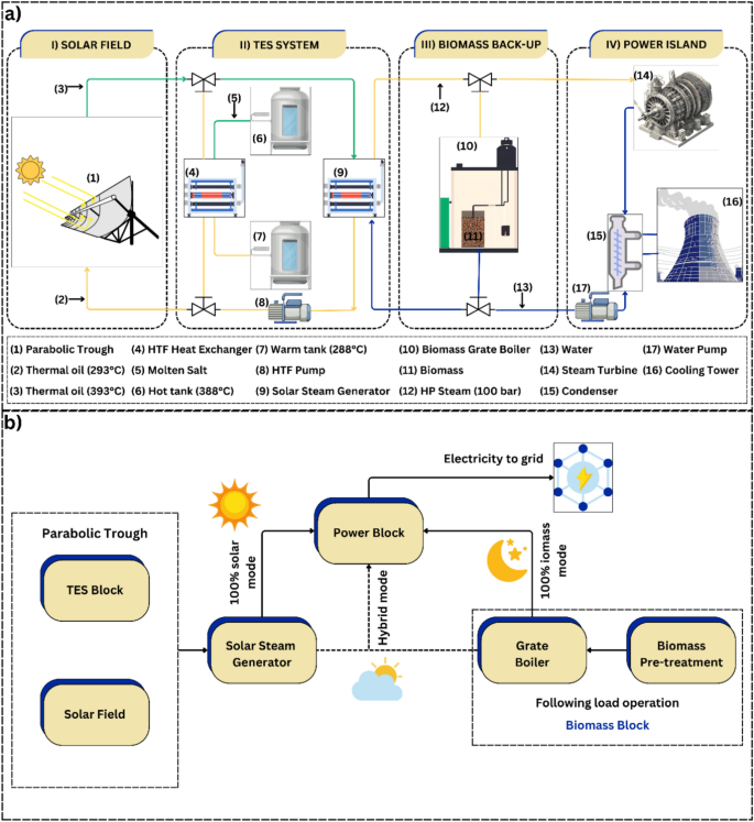
Mirrors are used in CSP systems to focus solar radiation and convert it into energy services like electricity, heat, or bioproducts. CSP technologies can be point-focused, like solar tower (ST) and parabolic dish (PD) systems, or linearly focused, like parabolic trough (PT) and linear Fresnel (LF) collectors, depending on the form of the sun reflection³. PT systems were chosen for this study due to their high maturity, current commercial deployment, and suitability for large-capacity TES systems like 2-tank molten salt storage (an indirect TES system (thermal oil—molten salts)). PT systems consist of parabolic-shaped mirrors and a receiver tube of the same length at the focal point, where a thermal fluid, e.g., water/steam, synthetic oil, or molten salts, is heated for energy storage or to drive a Rankine power cycle⁴⁶. As per Fig. 1a and b, the hybridized CSP-PT with a dual supporting system (biomass and TES) included four main components such as (i) the solar field, (ii) TES technology, (iii) biomass boiler combustion, and (iv) the power island. It is important to note that, the integration of TES enhances dispatchability, cost-efficiency, and environmental sustainability, enabling extended operational hours, improved grid stability, cogeneration capabilities, and scalability. This advancement positions TES as a viable solution for reducing reliance on fossil fuels, contributing to the development of highly efficient and sustainable energy systems¹⁸. Moreover, grate boilers are installed parallel to the power island for biomass combustion instead of fluidized bed boilers or biomass-based syngas combustion because of their advancement and simplicity^19,47. The cost of installing conventional CSP plants is generally high and a lack of organic materials (biomass backup system). Therefore, a 50 MW_e hybridized CSP-PT plant was built, combining two backup techniques (biomass and TES).

(a) Hybrid CSP-PT plant with biomass and TES systems, (b) simplified scheme of hybrid CSP-PT plant.

Full size image

In this study, three operations strategies were characterized by extensive intelligent models: PT-BC-NB, PT-OS1-MB, and PT-OS2-FB. Furthermore, the TES technology can extend the operational hours of the CSP-PT plant from 0 to 20 h with a 5-h step. The advantages of combining the CSP-PT plant with two backup systems (TES and biomass) can be summed up as follows: (i) a steady supply of electricity; (ii) increased plant efficiency; (iii) a reduction in greenhouse gas emissions; and (iv) flexibility to adapt to different climates and geographical locations.

Profitability factor (P_F)

This section outlines various financial indicators used to evaluate the economic performance of power plants according to the available literature. In common, the levelized cost of electricity (LCOE) was utilized frequently to assess the generating cost of multiple renewable power technologies, such as hybridized CSP-PT plants^6,48. As per Eq. (1), LCOE can be calculated based on several variables such as the capital costs of the hybridized CSP-PT plant, the plant’s operational lifetime, operational and maintenance costs, the biomass cost, the annual growth percentage, the discount rate, the output power, and the real discount percentage. Nevertheless, many researchers argue that LCOE is not the best metric because it overlooks fluctuations in electricity prices, does not accurately reflect the profitability of power supplied to the grid, and does not define the plant’s grid parity^49,50. Here, the LCOE measure is only considered when the predicted price of electricity is time-dependent. Therefore, new financial metrics have been proposed by multiple researchers to replace the limited LCOE, such as the net value of electricity (NVOE), the system LCOE, the Levelized value of electricity (LVOE)⁵¹, and the profitability-adjusted LCOE¹⁸. P_F is defined as a new financial metric that tackles the above limitations and can define the grid parity of a hybridized CSP-PT plant.

In this context, grid parity refers to the point at which the cost of generating electricity from renewable energy sources becomes ≤ the cost of purchasing electricity from the grid, typically from traditional fossil fuels⁵². Previously, LCOE’s economic analysis did not account for market electricity prices. The P_F metric extends to LCOE by incorporating this information. According to Eq. (2), P_F is the average of the calculated LCOE and the estimated hourly market price of electricity over the year. A positive P_F indicates gains over grid parity, while a negative P_F indicates losses. Tables 1 and 2 show the technical and financial parameters of the hybrid CSP-PT plant.

According to Eqs. 1 and 2; \({C}_{o}\) is the capital cost of the hybridized CSP-PT plant ($). \({C}_{n}\) is the annual operational and maintenance costs ($). \({F}_{n}\) is the annual biomass cost ($). \({i}_{n}\) is annual growth percentage (%). \(N\) is the plant’s operational lifetime (years). \({d}_{nomindal}\) is the nominal discount percentage (%), \({d}_{real}\) is the real discount percentage (%). \({Q}_{n}\) is the annual output power (MWh) and \({Q}_{h}\) is the hourly output power (MWh). \({PMIBEL}_{h}\) is the electricity market price ($/kWh), and \(H\) is the annual electricity generated hourly.

Materials and methods

Dataset and pre-processing

This study analyzed a dataset from two experimental papers for prediction analysis^3,18. The hybridized CSP-PT plant was chosen as a case study because it is well-developed, widely utilized commercially, and offers an opportunity to explore how solar fields, TES, and biomass backup can work together efficiently. The dataset, containing 10,000 records, included direct capital costs such as (power island, solar field, heat transfer fluid, TES, and biomass boiler) and other parameters such as (biomass cost annual escalation rate, hourly electricity price annual escalation rate, and peaks and troughs for daily electricity prices). The financial impact of the hybridized CSP-PT plant with two backup systems (TES and biomass) was predicted using these input factors.

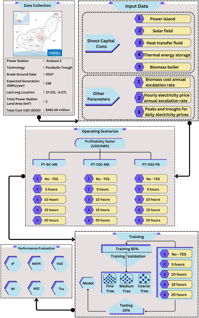
Several operational situations, including PT-BC-NB, PT-OS1-MB, and PT-OS2-FB, were used to predict P_F. 20% (2000 points) of the dataset was used for testing three alternative optimizers, while the remaining 80% (8000 points) was used for training. To guarantee a mean of 0 and a standard deviation of 1, the dataset was standardized during pre-processing using the standard scaler function (see Fig. 2).

Main steps of the research methodology.

Full size image

Decision tree optimizers

The decision tree (DT) is a widely utilized non-parametric model in supervised learning, demonstrating robust capabilities in both regression and classification tasks^53,54. The fundamental concept underlying DT involves constructing a binary tree through successive partitioning of dataset nodes, ultimately forming a hierarchical tree structure^55,56,57. These partitions, facilitated by decision-making panels, segment the dataset into smaller subgroups, representing the outcomes at the terminal leaf nodes.

Decision tree models are trained using a hierarchical tree-like structure, known as tree regression, to enable predictive capabilities. A DT includes three key node types: root, interior, and leaf nodes. The root node serves as the starting point, forming interior nodes defining the model’s structure and decision-making rules. The leaf nodes represent the final output or decision at each branch.

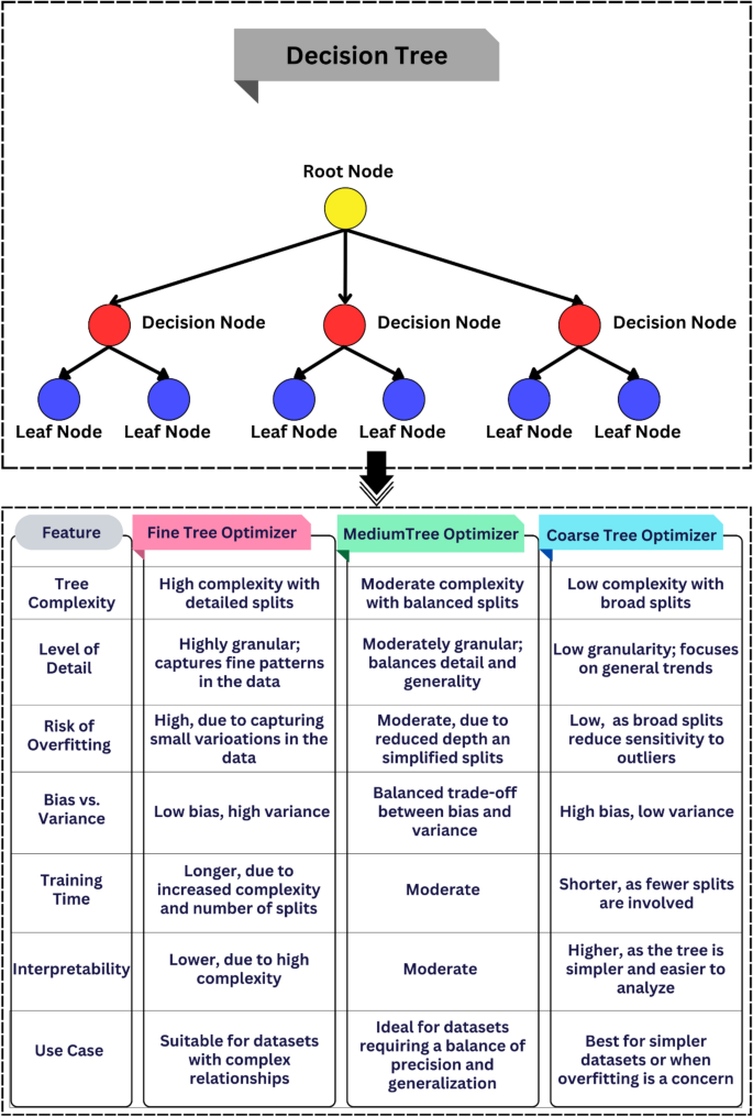
This study utilized the DT regressor from the scikit-learn library to train the model. The hierarchical structure of the DT is illustrated in Fig. 3, emphasizing its layered arrangement. Fine, medium, and coarse tree optimizers differ significantly in complexity, detail, and suitability for various datasets. Fine optimizers are highly complex, featuring detailed splits that capture intricate patterns in the data, but they are highly risky of overfitting, low interpretability, and longer training times. In contrast, medium optimizers offer a balanced trade-off, with moderate complexity and granularity, making them ideal for datasets requiring a blend of precision and generalization while maintaining a reasonable risk of overfitting and interpretability. Coarse optimizers are the most straightforward, employing broad splits that focus on general trends, resulting in low training times, minimal risk of overfitting, and high interpretability, but they may underperform in capturing finer details. The choice of optimizer depends on the dataset’s complexity, desired level of generalization, and acceptable bias-variance trade-off.

Simple representation of the decision optimizers regression architecture.

Full size image

Formulation and engineering of optimizers

Three decision tree optimizers were developed to predict the P_F of hybridized CSP-PT plants equipped with two backup systems (biomass and TES). The power plant was assessed under different operating scenarios, including PT-BC-NB, PT-OS1-MB, and PT-OS2-FB. The input variables included direct capital costs such as (power island, solar field, heat transfer fluid, thermal energy storage, and biomass boiler) and other parameters such as (biomass cost annual escalation rate, hourly electricity price annual escalation rate, and peaks and troughs for daily electricity prices). Furthermore, P_F was predicted to use various TES capacities, such as 0, 5, 10, 15, and 20 h.

The implementation of decision tree optimizers requires multiple steps. Step (1) determines the requirements for predicting accuracy and selecting suitable splits. Other crucial factors are selecting the best tree and determining when to stop splitting further⁵⁸. Initially, accuracy conditions can be defined by re-substitution, test samples, or cross-validation errors. Meanwhile, the re-substitution error is determined by employing the same dataset and utilized for making the predictor " \(p\)", as expressed below in Eq. (3):

Here, the learning samples are characterized as (\({u}_{i}\), \({v}_{i}\)). \(i = 1, 2, \dots , N\).

To calculate the error of cross-validation, sample \(X\) of size \(N\) is split into \(k\) sub-samples \({X}_{1}\), \({X}_{2}\), …, \({X}_{k}\) of almost the same sizes \({N}_{1}\), \({N}_{2}\), …, \({N}_{k1}\), respectively. The sub-sample \(X-{X}_{k}\) is utilized to build the predictor \(p.\) After, the cross-validation error is calculated from the sub-sample \({X}_{k}\) as explained in Eq. (4):

Here, \({p}^{\left(k\right)}\left({u}_{i}\right)\) is calculated from the sub-sample \(X.\) \({X}_{k}.\)

The test sample error is determined by splitting the total cases into two sub-samples, \({X}_{1}\) and \({X}_{2}\) with sizes \(N\) and \({N}_{2},\) respectively. Equation (5) is used to compute the test sample error.

Here, \({X}_{2}\) is the sub-sample not used in building the predictor (\(p\)).

Step (2) involves choosing appropriate splits to predict the values of the continuous dependent variable. Splits are evaluated with a node impurity measure, which provides insights into the relative homogeneity of cases inside terminal nodes. Equation (6) illustrates the calculation of a node’s impurity in a regression tree using the least-squared deviation.

Here, \({N}_{w}(t)\) represents the weighted number of cases in node \((t)\). \({w}_{i}\) is the weighting variable value for case \((i)\). \({f}_{i}\) is the frequency variable value. \({v}_{i}\) is the response variable value. \(\overline{v }(t)\) is the weighted mean for node \((t)\).

Step (3) sets the dividing criteria for dividing based on the minimum number of nodes. The final step is to select the optimal tree size through pruning, aiming for the most miniature tree with minimal effort to balance predictive performance and complexity.

Six regression metrics were used in this work to evaluate the performance of the decision tree models such as R² (R-squared), MAPE (Mean Absolute Percentage Error), WI (Willmott’s Index), KGE (Kling-Gupta Efficiency), NSE (Nash–Sutcliffe Efficiency), and U₉₅ (95^th Percentile Uncertainty)^59,60,61,62. The equations are written as below:

Here; \({y}_{i}\) is the experimental P_F and \({\widehat{y}}_{i}\) is predicted P_F. \(\overline{y}\) is the mean experimental P_F value. \(\Sigma\) represents the sum of all data points. \(r\) is the Pearson correlation coefficient between experimental and predicted values. \(\alpha\) is the ratio of the standard deviations of predicted to experimental values. \(\beta\) is the ratio of their means. \(\sigma\) denotes the standard deviation of the predicted values.

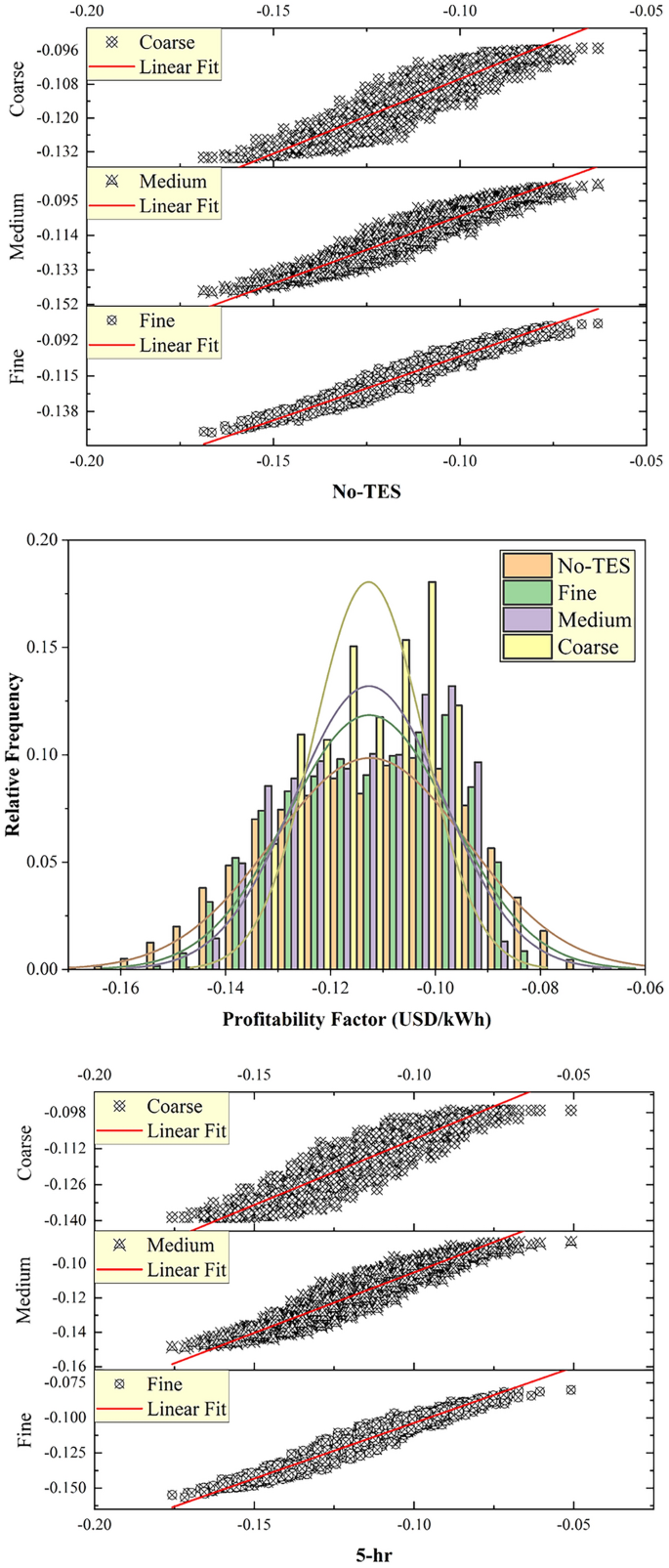
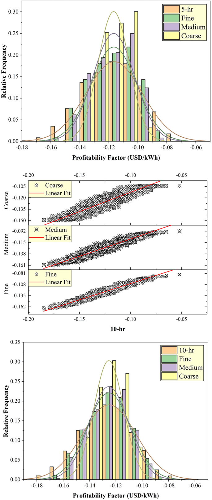
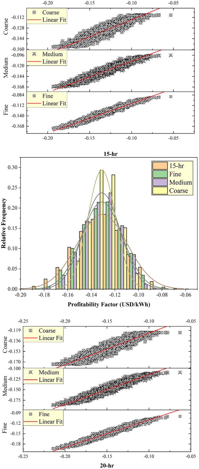
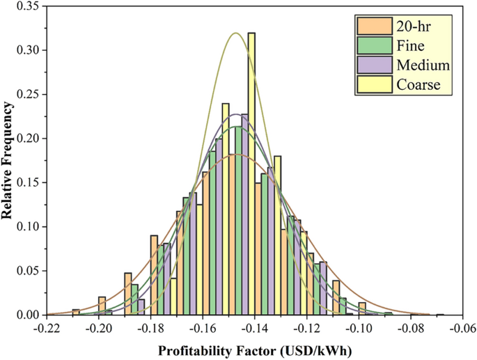
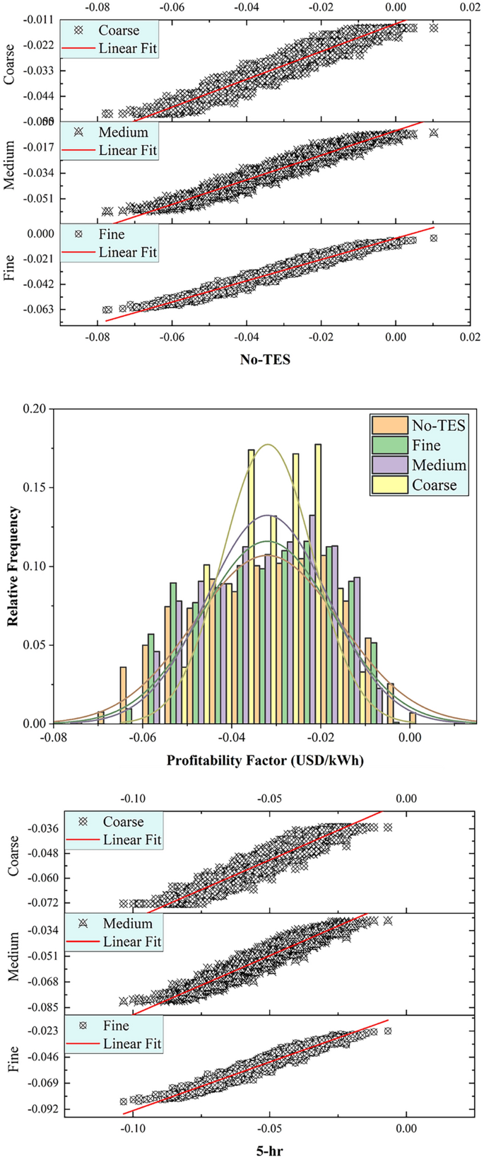
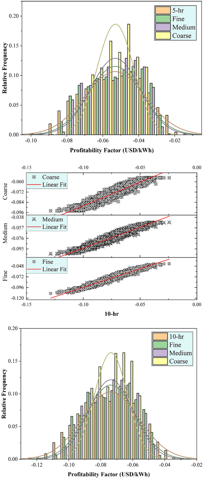
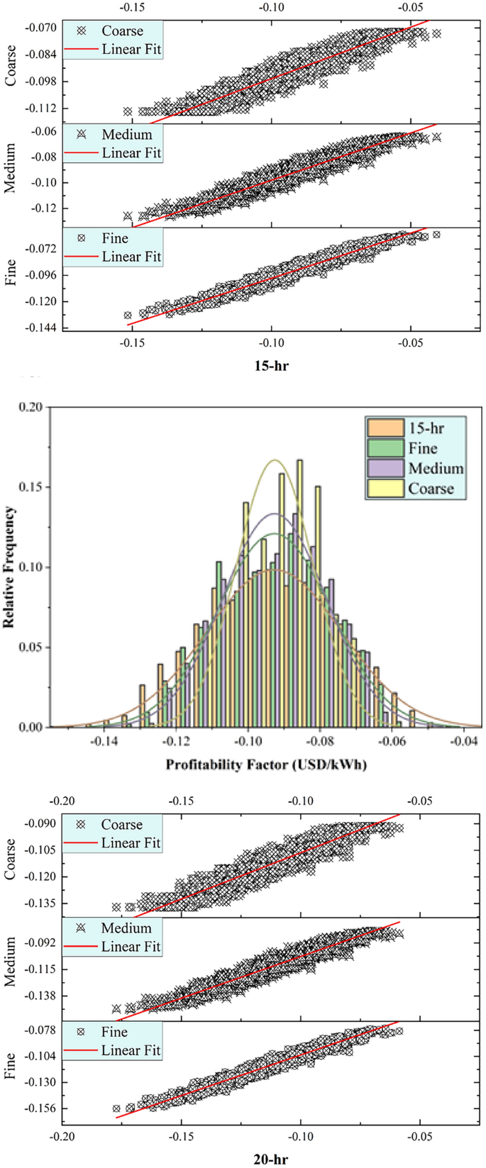
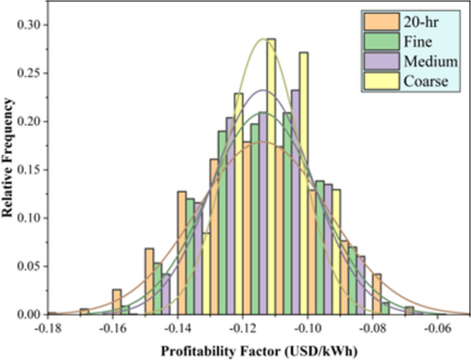
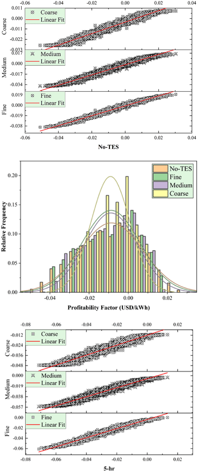
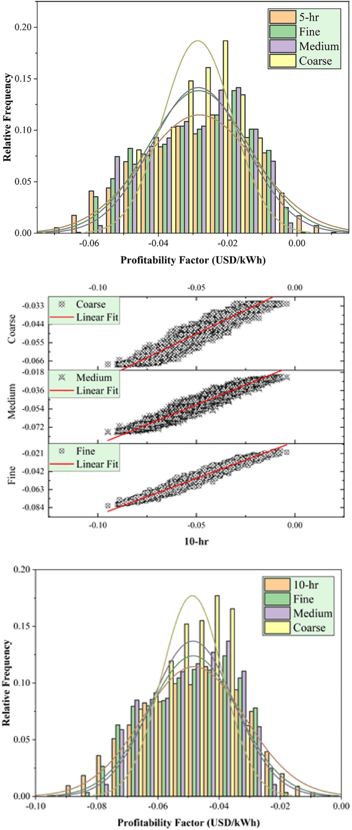
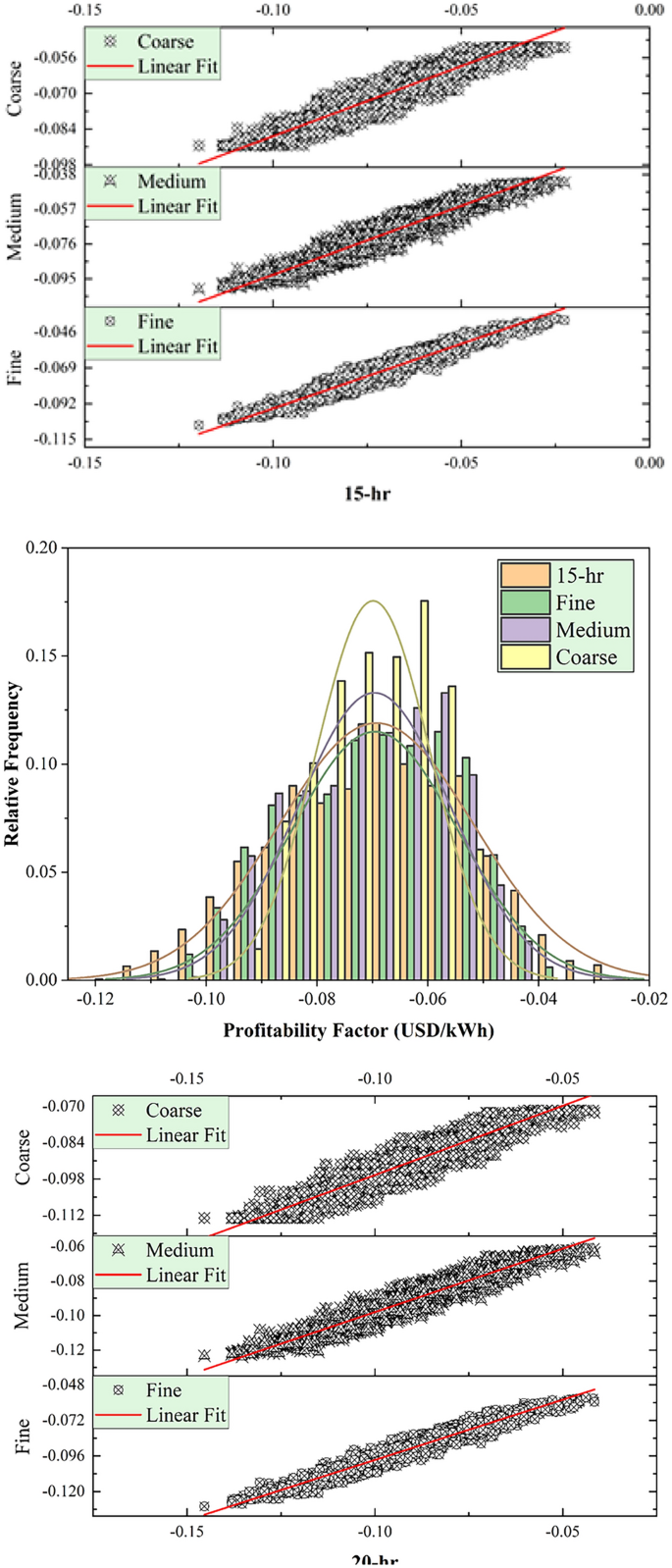
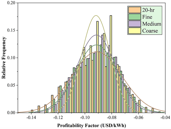
This section discussed the modeling performance using statistical metrics and graphical presentation, including scatter plots and relative frequency distribution of the testing results of the developed tree optimizers using PT-BC-NB, PT-OS1-MB, and PT-OS2-FB (Figs. 4, 5, 6). Figure 4 reported the determination coefficient R² and relative frequency distribution for the PT-BC-NB case across different TES capacities (No-TES, 5 h, 10 h, 15 h, 20 h) and various tree optimizers (fine, medium, coarse). Generally, as TES capacity increases, the R² values improved, suggesting enhanced predictive performance such as (0.946, 0.894, 0.744) for No-TES, (0.925, 0.865, 0.716) for 5 h, (0.927, 0.867, 0.715) for 10 h, (0.931, 0.872, 0.718) for 15 h and (0.933, 0.874, 0.720) for 20 h, using fine, medium, coarse optimizers, respectively. The (fine) model consistently yields higher R² values than the medium and coarse trees, indicating the ability of more detailed feature representations to capture patterns in the unseen data. Furthermore, relative frequency histograms examine the observed and predicted values’ central tendency, skew, and variability distributions. In conclusion, the analysis of 2,000 testing data points highlights distinct optimization behaviours. The fine optimizer achieves a symmetric, bell-shaped distribution, reflecting consistent performance. The coarse optimizer exhibits a multi-modal pattern, indicating distinct subgroups within the data. The medium optimizer strikes a balance, combining the fine optimizer’s symmetry with the coarse’s variability, capturing a broader range of data patterns. These results emphasize the trade-offs in optimization strategy selection.

Scatter plots and relative frequency distribution of PT-BC-NB.

Full size image

Scatter plots and relative frequency distribution of PT-OS1-MB.

Full size image

Scatter plots and relative frequency distribution of PT-OS2-FB.

Full size image

Figure 5 presented the R² and relative frequency distribution for PT-OS1-MB throughout different TES capacities (No-TES, 5 h, 10 h, 15 h, 20 h) and various tree optimizers (fine, medium, coarse). Generally, as the TES hour increases, the R² values decreased, such as (0.964, 0.934, 0.816) for No-TES, (0.946, 0.911, 0.789) for 5 h, (0.941, 0.900, 0.767) for 10 h, (0.938, 0.890, 0.750) for 15 h and (0.935, 0.883, 0.734) for 20 h, using fine, medium, coarse tree optimizers, respectively. The (fine) optimizer consistently yields higher R² values than the medium and coarse trees, indicating the ability of more detailed feature representations to capture patterns in the unseen data. In addition, relative frequency histograms revealed the observed and predicted values’ central tendency, skewness, and variability. In conclusion, with 2000 testing data points, the fine optimizer revealed a perfectly symmetric, bell-shaped distribution, while the coarse optimizer exhibits a multi-modal pattern indicating distinct subgroups. The medium tree optimizer falls between these extremes, capturing a balanced representation between the best and worst histogram shapes.

Figure 6 exhibited the R² and relative frequency distribution for PT-OS2-FB in various TES capacities (No-TES, 5 h, 10 h, 15 h, 20 h) and various tree optimizers (fine, medium, coarse). Generally, as TES capacity increased, the R² values decreased, such as (0.974, 0.949, 0.827) for No-TES, (0.958, 0.928, 0.808) for 5 h, (0.946, 0.907, 0.780) for 10 h, (0.937, 0.892, 0.760) for 15 h and (0.931, 0.879, 0.742) for 20 h, using fine, medium, coarse tree optimizers, respectively. The (fine) optimizer consistently yields higher R² values than the medium and coarse optimizers, indicating the ability of more detailed feature representations to capture patterns in the unseen data. Furthermore, relative frequency histograms demonstrate the observed and predicted values’ central tendency, skewness, and variability distributions. In conclusion, with 2000 testing data points, the fine optimizer reveals a perfectly symmetric, bell-shaped distribution, while the coarse optimizer exhibits a multi-modal pattern indicating distinct subgroups. The medium tree optimizer falls between these extremes, capturing a balanced representation between the best and worst histogram shapes.

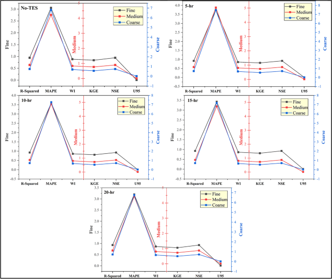
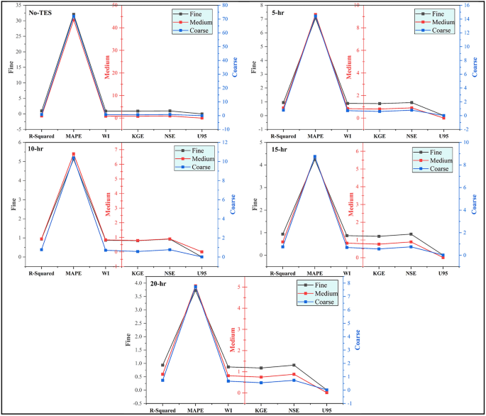
In Figs. 7, 8 and 9, the statistical metrics such as including R², MAPE, WI, KGE, NSE, and U₉₅ for PT-BC-NB, PT-OS1-MB, and PT-OS2-FB during the testing set were presented. The PT-BC-NB case’s performance was compared to multiple time storages (No-TES, 5 h, 10 h, 15 h, and 20 h) and various decision tree optimizers (fine, medium, coarse). Generally, all models showed good performance across all TES capacities, with R² values consistently > 0.9 (for fine), > 0.8 (for medium), and > 0.7 (for coarse), with WI values always > 0.85 (for fine), > 0.8 (for medium) and > 0.6 (for coarse), with NSE values consistently > 0.9 (for fine), > 0.8 (for medium) and > 0.7 (for coarse) and with KGE values consistently > 0.8 (for fine), > 0.7 (for medium) and > 0.5 (for coarse). Moreover, MAPE metrics show an average value of (3.409% for fine), (4.687% for medium) and (7.133% for coarse), indicating accurate predictions. In addition, U₉₅ values (Uncertainty in prediction) suggest that the model captures probability at upper percentiles with an average value of 0.0104 for fine, 0.0142 for medium, and 0.0211 for medium.

Statistical metrics of the PT-BC-NB.

Full size image

Statistical metrics of the PT-OS1-MB.

Full size image

Statistical metrics of the PT-OS2-FB.

Full size image

The fine tree optimizer consistently provides superior results compared to medium and coarse. A coarse tree optimizer has a higher MAPE and uncertainty and a lower R², WI, NSE, and KGE values, indicating difficulties in capturing prediction patterns. The tree optimizer performance decreases with increasing TES capacity. However, the model still maintains a satisfactory level of accuracy. The fine optimizer is ideal for achieving superior accuracy, particularly for short-term predictions.

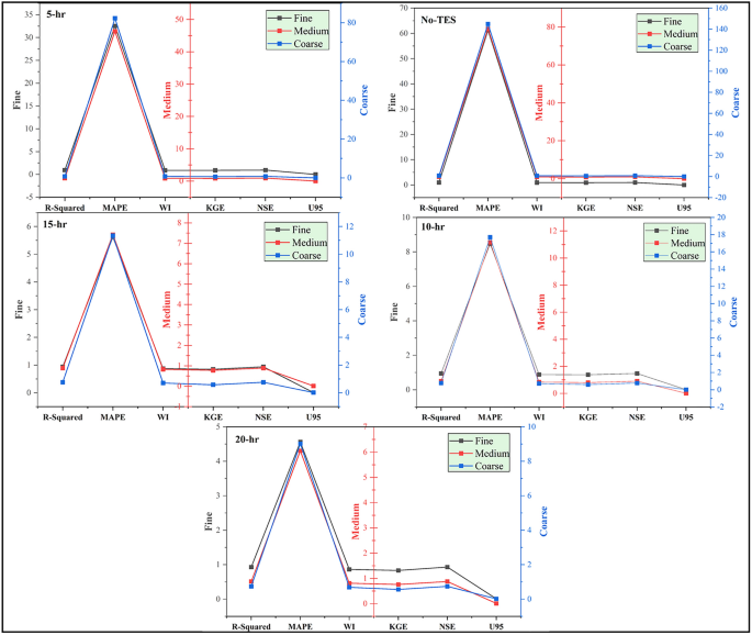
The PT-OS1-MB performance was evaluated across multiple TES capacitates (No-TES, 5 h, 10 h, 15 h, and 20 h) and various tree optimizers (fine, medium, coarse) using R², MAPE, WI, KGE, NSE, and U₉₅ metrics. Generally, all tree models showed good performance across the five TES capacitates, with R² values consistently > 0.93 (for fine), > 0.88 (for medium), and > 0.73 (for coarse), with WI values always > 0.86 (for fine), > 0.81 (for medium) and > 0.67 (for coarse), with NSE values consistently > 0.93 (for fine), > 0.88 (for medium) and > 0.73 (for coarse) and with KGE values always > 0.82 (for fine), > 0.74 (for medium) and > 0.55 (for coarse). Furthermore, MAPE metrics are relatively low in the average value of (10.446% for fine), (14.038% for medium) and (22.685% for coarse), indicating accurate predictions, while U₉₅ values (Uncertainty in prediction) suggest the model captures probability at upper percentiles with an average value of 0.0083 for fine, 0.0110 for medium and 0.0169 for medium, respectively.

The fine tree optimizer was consistently superior to the medium and coarse models. The coarse optimizer has a greater MAPE, uncertainty, and lower R², WI, NSE, and KGE values, indicating difficulty capturing predictive characteristics. The tree model performance usually decreases as TES duration times increase, but the model maintains good accuracy. The fine tree optimizer is suitable for improving accuracy, particularly for long-term storage.

The PT-OS2-FB performance was evaluated using R², MAPE, WI, KGE, NSE, and U₉₅ across multiple TES capacities (No-TES, 5 h, 10 h, 15 h, and 20 h) and various decision tree optimization systems (fine, medium, coarse). Generally, all models showed good performance across the five TES capacities, with R² values consistently > 0.93 (for fine), > 0.87 (for medium), and > 0.74 (for coarse), with WI values always > 0.86 (for fine), > 0.81 (for medium) and > 0.68 (for coarse), with NSE values consistently > 0.93 (for fine), > 0.87 (for medium) and > 0.74 (for coarse) and with KGE values always > 0.83 (for fine), > 0.76 (for medium) and > 0.56 (for coarse). Moreover, MAPE metrics are relatively low in the average value of (22.479% for fine), (30.018% for medium) and (53.058% for coarse), indicating accurate predictions, while U₉₅ values (Uncertainty in prediction) suggest the model captures probability at upper percentiles with an average value of 0.0075 for fine, 0.0099 for medium and 0.0155 for medium, respectively.

The fine tree optimizer consistently achieves superior results than the medium and coarse models. MAPE and uncertainty and lower R², WI, NSE, and KGE values suggest a coarse model with difficulty capturing predictive patterns. Although the model’s accuracy remains satisfactory, the algorithm’s performance declines as TES length times increase. In summary, the fine optimizer is the most suitable choice for increasing accuracy, particularly for short-term storage.

The development of tree optimizers to estimate the P_F of CSP plants with a dual supporting system (biomass and TES) is a significant step in enhancing the utilization of solar energy materials. This work focuses on enhancing the following: (1) dispatchability and reliability: CSP-biomass hybrids provide continuous power by using TES and biomass as backup, addressing solar intermittency. (2) Economic viability through the P_F estimation: The P_F parameter provides insights into financial performance under various scenarios, guiding cost-effective decisions and boosting the market penetration of solar materials. (3) The use of solar energy materials: Evaluating different scenarios helps refine CSP technologies, enhancing the efficiency of mirrors, receivers, and heat transfer fluids, and reducing costs. (4) This study promotes CSP-biomass integration, promoting the wider adoption of solar technologies in diverse regions with different solar and biomass resources. (5) CSP-biomass hybrids integrate renewable energy sources, cutting carbon emissions and advancing the development of sustainable solar materials for a low-carbon future. (6) P_F insights support policymakers and investors in developing CSP-biomass plants, fostering policies and investments that accelerate technological advancements in solar materials.

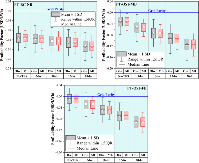
Figure 10 illustrates the differences between the experimental and predicted P_F for PT-BC-NB, PT-OS1-MB, and PT-OS2-FB under five different TES capacities (No-TES, 5 h, 10 h, 15 h, and 20 h) using the fine tree optimizer. It is essential to emphasize that the excessive stochasticity and nonlinearity of duplicated input parameters in the machine learning matrix make it difficult to develop a basic computer aid model for this complex system. Figure 10 indicates that most P_F values seemed less than zero with a slight negative value. Grid parity is achieved when the cost of generating power from a specific source, such as a solar system with energy storage and biomass backup, becomes lower than the cost of purchasing electricity from the grid. In a hybrid CSP plant with a dual supporting system (biomass and TES), the cost of system installation and operation is either the same or less expensive than purchasing electricity from the grid.

Experimental and predicted P_F using fine optimizer: PT-BC-NB, PT-OS1-MB, and PT-OS2-FB.

Full size image

The balance between biomass use and TES capacity profoundly impacts the economic and technical efficacy of concentrated solar power parabolic trough (CSP-PT) systems. Figure 10 shows that increasing the share of the biomass backup system improves profitability, whilst increased TES capacity has the reverse effect. For example, the PT-OS2-FB-No TES arrangement has a 95% chance of increasing sales from $0.095 to $0.114 per kWh. However, expanding the TES capacity from 0 to 20 h diminishes this incremental income by an average of 52%. Despite the financial limits imposed by TES, the PT-OS1-MB design offers the possibility of a more consistent energy supply. In contrast, for PT-OS2-FB, increased TES capacity reduces supply-side uncertainties associated with biomass, potentially lowering total yearly biomass consumption by up to 55% (equal to 109 kilotons). These findings highlight the important role of maximizing biomass and TES capacity to balance economic returns and operational reliability in CSP–PT systems.

This study predicted a new economic metric, the Profitability Factor (P_F), for hybridized CSP-PT plants using fine, medium, and coarse decision tree optimizers. Three operational scenarios (PT-BC-NB, PT-OS1-MB, and PT-OS2-FB) with five different TES hour capabilities (No-TES, 5 h, 10 h, 15 h, and 20 h) were used to determine the P_F. The dataset comprised various input parameters, including direct capital costs (power island, solar field, heat transfer fluid, thermal energy storage, and biomass boiler), as well as additional factors such as the annual escalation rate of biomass costs, the annual escalation rate of hourly electricity prices, and the daily fluctuations in electricity prices. The key findings of this study are summarized as follows:

1. i.

   The PT-BC-NB scenario showed strong performance across statistical metrics. Fine, medium, and coarse tree optimizers achieved R² values > 0.9, > 0.8, and > 0.7, respectively. WI scores were > 0.85 (fine optimizer), > 0.8 (medium optimizer), and > 0.6 (coarse optimizer). NSE values exceeded 0.9 (fine optimizer), 0.8 (medium optimizer), and 0.7 (coarse optimizer), while KGE values were > 0.8 (fine optimizer), > 0.7 (medium optimizer), and > 0.5 (coarse optimizer). MAPE was low, at 3.409 (fine optimizer), 4.687 (medium optimizer), and 7.133 (coarse optimizer). Uncertainty (U₉₅) was effective with values of 0.0104 (fine optimizer), 0.0142 (medium optimizer), and 0.0211 (coarse optimizer).

2. ii.

   The PT-OS1-MB scenario demonstrated strong and consistent performance. Fine, medium, and coarse tree optimizers achieved R² values > 0.93, > 0.88, and > 0.73, respectively. WI scores were > 0.86 (fine optimizer), > 0.81 (medium optimizer), and > 0.67 (coarse optimizer). NSE values exceeded 0.93 (fine), 0.88 (medium), and 0.73 (coarse), while KGE values were > 0.82 (fine optimizer), > 0.74 (medium optimizer), and > 0.55 (coarse optimizer). MAPE was low, at 10.446 (fine optimizer), 14.038 (medium optimizer), and 22.685 (coarse optimizer). Uncertainty (U₉₅) was effective, averaging 0.0083 (fine optimizer), 0.0110 (medium optimizer), and 0.0169 (coarse optimizer).

3. iii.

   The PT-OS2-FB scenario exhibited high performance across all metrics. Fine, medium, and coarse tree optimizers achieved R² values > 0.93, > 0.87, and > 0.74, respectively. WI scores were > 0.86 (fine optimizer), > 0.81 (medium optimizer), and > 0.68 (coarse optimizer). NSE values exceeded 0.93 (fine optimizer), 0.87 (medium optimizer), and 0.74 (coarse optimizer), while KGE values were > 0.83 (fine optimizer), > 0.76 (medium optimizer), and > 0.56 (coarse optimizer). MAPE values were low, at 22.479 (fine optimizer), 30.018 (medium optimizer), and 53.058 (coarse optimizer). Uncertainty (U₉₅) was effective, averaging 0.0075 (fine optimizer), 0.0099 (medium optimizer), and 0.0155 (coarse optimizer).

4. iv.

   The PT-OS2-FB-No TES configurations exhibited exceptional performance, with a 95% probability of generating additional revenues in the range of $0.095 to $0.114 per kWh.

5. v.

   The increase in the TES hour capacity resulted in an average reduction of 52% in additional revenues.

6. vi.

   The PT-OS2-FB scenario provided an opportunity to reduce uncertainty in biomass supply, resulting in potential savings of up to 55% of the total annual consumption, equivalent to 109 kt/year.

Future research on CSP-biomass hybrid power plants should focus on several critical areas to enhance their design, performance, and sustainability. One significant topic is studying different machine learning techniques to increase prediction accuracy, notably by combining variables linked to biomass supply and variations. Expanding research to include hybrid CSP technologies beyond parabolic trough systems is equally important, allowing for a greater understanding of their applicability and efficiency. Furthermore, conducting long-term performance analyses is essential for evaluating these systems’ sustainability and financial benefits. A comparative analysis of the LCOE should also be included, despite the acknowledged advantages of the P_F in assessing system performance. Many existing solar thermal systems are primarily evaluated using LCOE, and this metric will facilitate meaningful comparisons and decision-making for researchers and stakeholders. Furthermore, carbon emissions from biofuel backup systems should be examined in detail, including the calculation of CO₂ emissions under various scenarios and TES durations. The combustion of biogas, typically represented by the equation (\({CH}_{4}+{2O}_{2}\to {CO}_{2}+{2H}_{2}O),\) releases specific amounts of CO₂ based on operational conditions. Quantifying these emissions is critical for assessing the environmental impact and sustainability of CSP-biomass systems.

Considering CO₂ emissions from biogas systems as a cost function, it is a potential avenue for future research. This approach could provide more insights into the economic and environmental trade-offs associated with biofuel use, providing a more holistic assessment of system performance. Researchers are encouraged to explore this topic to develop innovative strategies for reducing emissions and reducing costs.

Finally, using exergy analysis in the study of CSP-biomass hybrid power plants could significantly contribute to understanding energy efficiency and losses within the system. Future research should prioritize exergy-based evaluations to identify potential improvements in design and operation, ensuring these hybrid systems continue to evolve as clean, efficient, and economically viable energy solutions.

ANNs:

Artificial neural networks

BC:

Base case

BDSCA:

Balance-dynamic sine–cosine

CF:

Capacity factor

CHP:

Combined heat and power plant

CSP:

Concentrating solar power

R² :

Coefficient of determination

DCCN:

Deep convolutional neural networks

DCC:

Direct capital cost

DNI:

Direct normal irradiance (kWh/m²/year)

DRE:

Dispatchable renewable energy

DT:

Decision tree

EPC:

Energy performance contract

FB:

Full biomass

HTF:

Heat transfer fluid

IPH:

Industrial process heat

KGE:

Kling–Gupta efficiency

LCOE:

Levelized cost of electricity

LVOE:

Levelized value of electricity

LSTM:

Long short-term memory

MAPE:

Mean absolute percentage error

MB:

Medium biomass

MLP:

Multi-layer perceptron

NB:

No Biomass

NREL:

National Renewable Energy Laboratory

NSE:

Nash–Sutcliffe Efficiency

NVOE:

Net value of electricity

NRMSE:

Normalized Root Mean Square Error

ORC:

Organic Rankine cycle

OS1:

Operation strategy 1

OS2:

Operation strategy 2

PD:

Parabolic dish

PPA:

Power purchase agreement

PT:

Parabolic trough

PCM:

Phase change material

RF:

Random forest

SDA:

Swarm decomposition algorithm

SCA:

Solar collector arrays

SM:

Solar multiple

ST:

Solar tower

TES:

Thermal energy storage

VRE:

Variable renewable energy

VMD:

Variation mode decomposition

WI:

Willmott’s Index

C _n :

Operation and maintenance costs ($/year)

C _o :

Capital cost ($)

\({d}_{nomindal}\) :

Nominal discount rate (%)

\({d}_{real}\) :

Real discount rate (%)

F _n :

Biomass costs ($/year)

H:

Annual number of generation hours

i _n :

Annual escalation value (%)

N :

Power plant useful life (years)

P _F :

Profitability factor ($/kWh)

\({PMIBEL}_{h}\) :

Hourly electricity price in MIBEL ($/kWh)

\({Q}_{h}\) :

Hourly power output (MWh)

\({Q}_{n}\) :

Plant power output (MWh/year)

1. Gielen, D. et al. The role of renewable energy in the global energy transformation. Energ. Strat. Rev. 24, 38–50 (2019).

   Article  MATH  Google Scholar 

2. Bouckaert, S. et al. Net zero by 2050: A roadmap for the global energy sector (2021).

3. Gutiérrez, R. E., Haro, P. & Gómez-Barea, A. Techno-economic and operational assessment of concentrated solar power plants with a dual supporting system. Appl. Energy 302, 117600 (2021).

   Article  MATH  Google Scholar 

4. Guerra, K., Haro, P., Gutiérrez, R. & Gómez-Barea, A. Facing the high share of variable renewable energy in the power system: Flexibility and stability requirements. Appl. Energy 310, 118561 (2022).

   Article  Google Scholar 

5. Gandhi, O., Kumar, D. S., Rodríguez-Gallegos, C. D. & Srinivasan, D. Review of power system impacts at high PV penetration Part I: Factors limiting PV penetration. Solar Energy 210, 181–201 (2020).

   Article  ADS  Google Scholar 

6. Pramanik, S. & Ravikrishna, R. A review of concentrated solar power hybrid technologies. Appl. Therm. Eng. 127, 602–637 (2017).

   Article  MATH  Google Scholar 

7. Huang, H. et al. Biomass briquette fuel, boiler types and pollutant emissions of industrial biomass boiler: A review. Particuology 77, 79–90 (2023).

   Article  CAS  MATH  Google Scholar 

8. Del Río, P., Peñasco, C. & Mir-Artigues, P. An overview of drivers and barriers to concentrated solar power in the European union. Renew. Sustain. Energy Rev. 81, 1019–1029 (2018).

   Article  Google Scholar 

9. Gani, A. et al. Analysis of technological developments and potential of biomass gasification as a viable industrial process: A review. Case Stud. Chem. Environ. Eng. 8, 100439 (2023).

   Article  MATH  Google Scholar 

10. González, C. A. D. & Sandoval, L. P. Sustainability aspects of biomass gasification systems for small power generation. Renew. Sustain. Energy Rev. 134, 110180 (2020).

    Article  MATH  Google Scholar 

11. Pantaleo, A. M. et al. Novel hybrid CSP-biomass CHP for flexible generation: Thermo-economic analysis and profitability assessment. Appl. Energy 204, 994–1006 (2017).

    Article  ADS  MATH  Google Scholar 

12. Pantaleo, A. M. et al. Hybrid solar-biomass combined Brayton/organic Rankine-cycle plants integrated with thermal storage: Techno-economic feasibility in selected Mediterranean areas. Renew. Energy 147, 2913–2931 (2020).

    Article  MATH  Google Scholar 

13. Powell, K. M., Rashid, K., Ellingwood, K., Tuttle, J. & Iverson, B. D. Hybrid concentrated solar thermal power systems: A review. Renew. Sustain. Energy Rev. 80, 215–237 (2017).

    Article  Google Scholar 

14. Milani, R., Szklo, A. & Hoffmann, B. S. Hybridization of concentrated solar power with biomass gasification in Brazil’s semiarid region. Energy Conv. Manag. 143, 522–537 (2017).

    Article  ADS  MATH  Google Scholar 

15. Mendoza, J. M. F. & Ibarra, D. Technology-enabled circular business models for the hybridisation of wind farms: Integrated wind and solar energy, power-to-gas and power-to-liquid systems. Sustain. Prod. Consum. (2023).

16. Peterseim, J. H., White, S., Tadros, A. & Hellwig, U. Concentrating solar power hybrid plants—Enabling cost effective synergies. Renew. Energy 67, 178–185 (2014).

    Article  Google Scholar 

17. Morell, D. CSP BORGES The World’s First CSP Plant Hybridized With Biomass (CSP Today, USA, 2012).

    MATH  Google Scholar 

18. Gutiérrez-Alvarez, R., Guerra, K. & Haro, P. Market profitability of CSP-Biomass hybrid power plants: Towards a firm supply of renewable energy. Appl. Energy 335, 120754 (2023).

    Article  MATH  Google Scholar 

19. Peterseim, J. H., White, S., Tadros, A. & Hellwig, U. Concentrated solar power hybrid plants, which technologies are best suited for hybridisation?. Renew. Energy 57, 520–532 (2013).

    Article  Google Scholar 

20. Servert, J., San Miguel, G. & Lopez, D. Hybrid solar-biomass plants for power generation; Technical and economic assessment. Global NEST Journal 13, 266–276 (2011).

21. Srinivas, T. & Reddy, B. Hybrid solar–biomass power plant without energy storage. Case Stud. Therm. Eng. 2, 75–81 (2014).

    Article  Google Scholar 

22. Peterseim, J. H., Tadros, A., Hellwig, U. & White, S. Increasing the efficiency of parabolic trough plants using thermal oil through external superheating with biomass. Energy Conv. Manag. 77, 784–793 (2014).

    Article  ADS  Google Scholar 

23. Bai, Z. et al. Thermodynamic evaluation of a novel solar-biomass hybrid power generation system. Energy Conv. Manag. 142, 296–306 (2017).

    Article  ADS  MATH  Google Scholar 

24. Peterseim, J. et al. Solar tower-biomass hybrid plants–maximizing plant performance. Energy Proc. 49, 1197–1206 (2014).

    Article  Google Scholar 

25. Middelhoff, E. et al. Hybrid concentrated solar biomass (HCSB) plant for electricity generation in Australia: Design and evaluation of techno-economic and environmental performance. Energy Conv. Manag. 240, 114244 (2021).

    Article  MATH  Google Scholar 

26. Wang, Y., Lou, S., Wu, Y., Miao, M. & Wang, S. Operation strategy of a hybrid solar and biomass power plant in the electricity markets. Electric Power Syst. Res. 167, 183–191 (2019).

    Article  MATH  Google Scholar 

27. Jian, P., Hu, W., Valipour, E. & Nojavan, S. Risk analysis of integrated biomass and concentrated solar system using downside risk constraint procedure. Solar Energy 238, 44–59 (2022).

    Article  ADS  MATH  Google Scholar 

28. Guo, X., Guo, Q., Valipour, E. & Nojavan, S. Risk assessment of integrated concentrated solar system and biomass using stochastic dominance method. Solar Energy 235, 62–72 (2022).

    Article  ADS  MATH  Google Scholar 

29. Segarra, J., Pérez, E., Moya, E., Ayuso, P. & Beltrán, H. Deep learning-based forecasting of aggregated CSP production. Math. Comput. Simul. 184, 306–318 (2020).

    Article  MathSciNet  Google Scholar 

30. Milidonis, K. et al. Review of application of AI techniques to solar tower systems. Solar Energy 224, 500–515 (2021).

    Article  ADS  MATH  Google Scholar 

31. Carballo, J. A., Bonilla, J., Berenguel, M., Fernández-Reche, J. & García, G. New approach for solar tracking systems based on computer vision, low cost hardware and deep learning. Renew. Energy 133, 1158–1166 (2019).

    Article  Google Scholar 

32. Zaaoumi, A. et al. Estimation of the energy production of a parabolic trough solar thermal power plant using analytical and artificial neural networks models. Renewable Energy 170, 620–638 (2021).

    Article  MATH  Google Scholar 

33. Boukelia, T., Arslan, O. & Mecibah, M. Potential assessment of a parabolic trough solar thermal power plant considering hourly analysis: ANN-based approach. Renew. Energy 105, 324–333 (2017).

    Article  Google Scholar 

34. Boukelia, T., Ghellab, A., Laouafi, A., Bouraoui, A. & Kabar, Y. Cooling performances time series of CSP plants: Calculation and analysis using regression and ANN models. Renew. Energy 157, 809–827 (2020).

    Article  Google Scholar 

35. May Tzuc, O. et al. Modeling and optimization of a solar parabolic trough concentrator system using inverse artificial neural network. J. Renew. Sustain. Energy 9, 013701 (2017).

    Article  MATH  Google Scholar 

36. Qi, Y. et al. Optimal configuration of concentrating solar power in multienergy power systems with an improved variational autoencoder. Appl. Energy 274, 115124 (2020).

    Article  MATH  Google Scholar 

37. Martinek, J. & Wagner, M. J. Efficient prediction of concentrating solar power plant productivity using data clustering. Solar Energy 224, 730–741 (2021).

    Article  ADS  MATH  Google Scholar 

38. Djaafari, A. et al. Hourly predictions of direct normal irradiation using an innovative hybrid LSTM model for concentrating solar power projects in hyper-arid regions. Energy Rep. 8, 15548–15562 (2022).

    Article  MATH  Google Scholar 

39. Alghamdi, H. et al. Machine learning model for transient exergy performance of a phase change material integrated-concentrated solar thermoelectric generator. Appl. Therm. Eng. 228, 120540 (2023).

    Article  MATH  Google Scholar 

40. Masero, E., Ruiz-Moreno, S., Frejo, J. R. D., Maestre, J. M. & Camacho, E. F. A fast implementation of coalitional model predictive controllers based on machine learning: Application to solar power plants. Eng. Appl. Artif. Intell. 118, 105666 (2023).

    Article  MATH  Google Scholar 

41. Sun, Y., Li, H.-W., Wang, D. & Du, C.-H. A novel zero emission combined power and cooling system for concentrating solar power: Thermodynamic and economic assessments and optimization. Case Stud. Therm. Eng. 58, 104406 (2024).

    Article  Google Scholar 

42. Ouali, H. A. L., Touili, S., Merrouni, A. A. & Moukhtar, I. Artificial neural network-based LCOH estimation for concentrated solar power plants for industrial process heating applications. Appl. Therm. Eng. 236, 121810 (2024).

    Article  Google Scholar 

43. Guermoui, M., Arrif, T., Belaid, A., Hassani, S. & Bailek, N. Enhancing direct Normal solar Irradiation forecasting for heliostat field applications through a novel hybrid model. Energy Conv. Manag 304, 118189 (2024).

    Article  Google Scholar 

44. Alawi, O. A. & Yaseen, Z. M. Data-driven based financial analysis of concentrated solar power integrating biomass and thermal energy storage: A profitability perspective. Biomass and Bioenergy 188, 107306 (2024).

    Article  Google Scholar 

45. Lovegrove, K. & Stein, W. in Concentrating Solar Power Technology 3–17 (Elsevier, 2021).

46. Peterseim, J. H., Hellwig, U., Tadros, A. & White, S. Hybridisation optimization of concentrating solar thermal and biomass power generation facilities. Solar Energy 99, 203–214 (2014).

    Article  ADS  Google Scholar 

47. Mohammadi, K., Saghafifar, M., Ellingwood, K. & Powell, K. Hybrid concentrated solar power (CSP)-desalination systems: A review. Desalination 468, 114083 (2019).

    Article  CAS  Google Scholar 

48. Mai, T., Mowers, M. & Eurek, K. Competitiveness metrics for electricity system technologies. (National Renewable Energy Lab. (NREL), Golden, CO (United States), 2021).

49. Musi, R. et al. in AIP Conference Proceedings. (AIP Publishing).

50. Ueckerdt, F., Hirth, L., Luderer, G. & Edenhofer, O. System LCOE: What are the costs of variable renewables?. Energy 63, 61–75 (2013).

    Article  Google Scholar 

51. Munoz, L. H., Huijben, J., Verhees, B. & Verbong, G. The power of grid parity: A discursive approach. Technol. Forecast. Soc. Change 87, 179–190 (2014).

    Article  MATH  Google Scholar 

52. Kadavi, P. R., Lee, C.-W. & Lee, S. Landslide-susceptibility mapping in Gangwon-do, South Korea, using logistic regression and decision tree models. Environ. Earth Sci. 78, 1–17 (2019).

    Article  MATH  Google Scholar 

53. Ferro, M., Silva, G. D., de Paula, F. B., Vieira, V. & Schulze, B. Towards a sustainable artificial intelligence: A case study of energy efficiency in decision tree algorithms. Concurr. Comput. Pract. Exp., e6815 (2021).

54. Asadollah, S. B. H. S., Sharafati, A., Motta, D. & Yaseen, Z. M. River water quality index prediction and uncertainty analysis: A comparative study of machine learning models. J. Environ. Chem. Eng. 9, 104599 (2021).

    Article  CAS  MATH  Google Scholar 

55. Nsangou, J. C. et al. Explaining household electricity consumption using quantile regression, decision tree and artificial neural network. Energy 250, 123856 (2022).

    Article  MATH  Google Scholar 

56. Jumin, E., Basaruddin, F. B., Yusoff, Y. B. M., Latif, S. D. & Ahmed, A. N. Solar radiation prediction using boosted decision tree regression model: A case study in Malaysia. Environ. Sci. Pollut. Res. 28, 26571–26583 (2021).

    Article  Google Scholar 

57. Swetapadma, A. & Yadav, A. A novel decision tree regression-based fault distance estimation scheme for transmission lines. IEEE Trans. Power Deliv. 32, 234–245 (2016).

    Article  MATH  Google Scholar 

58. Bhagat, S. K. et al. Wind speed prediction and insight for generalized predictive modeling framework: A comparative study for different artificial intelligence models. Neural Comput. Appl. 36, 14119–14150 (2024).

    Article  MATH  Google Scholar 

59. Alawi, O. A., Kamar, H. M. & Yaseen, Z. M. Optimizing building energy performance predictions: A comparative study of artificial intelligence models. J. Build. Eng. 88, 109247 (2024).

    Article  MATH  Google Scholar 

60. Pande, C. B. et al. Daily scale air quality index forecasting using bidirectional recurrent neural networks: Case study of Delhi India. Environ. Pollut. 351, 124040 (2024).

    Article  CAS  PubMed  MATH  Google Scholar 

61. Yaseen, Z. M. et al. Development of advanced data-intelligence models for radial gate discharge coefficient prediction: Modeling different flow scenarios. Water Resour. Manag. 37, 5677–5705 (2023).

    Article  MATH  Google Scholar 

Download references

Authors and Affiliations

1. Civil and Environmental Engineering Department, King Fahd University of Petroleum & Minerals, 31261, Dhahran, Saudi Arabia

   Zaher Mundher Yaseen

2. Interdisciplinary Research Centre for Membranes and Water Security, King Fahd University of Petroleum & Minerals, 31261, Dhahran, Saudi Arabia

   Zaher Mundher Yaseen

3. Department of Thermofluids, School of Mechanical Engineering, Universiti Teknologi Malaysia, 81310 UTM, Skudai, Johor Bahru, Malaysia

   Omer A. Alawi

4. Department of Power Mechanics Engineering Techniques, Technical Engineering College, Al-Bayan University, Baghdad, 10011, Iraq

   Omer A. Alawi

Contributions

ZMY: Conceptualization, supervision, project leader, validation investigation, analysis, writing up, revision. OAA: Conceptualization, supervision, modelling, project leader, validation investigation, analysis, writing up, revision.

Corresponding author

Correspondence to Zaher Mundher Yaseen.

Competing interests

The authors declare no competing interests.

Publisher’s note

Springer Nature remains neutral with regard to jurisdictional claims in published maps and institutional affiliations.

Open Access This article is licensed under a Creative Commons Attribution-NonCommercial-NoDerivatives 4.0 International License, which permits any non-commercial use, sharing, distribution and reproduction in any medium or format, as long as you give appropriate credit to the original author(s) and the source, provide a link to the Creative Commons licence, and indicate if you modified the licensed material. You do not have permission under this licence to share adapted material derived from this article or parts of it. The images or other third party material in this article are included in the article’s Creative Commons licence, unless indicated otherwise in a credit line to the material. If material is not included in the article’s Creative Commons licence and your intended use is not permitted by statutory regulation or exceeds the permitted use, you will need to obtain permission directly from the copyright holder. To view a copy of this licence, visit http://creativecommons.org/licenses/by-nc-nd/4.0/.

Reprints and permissions