When Amazon Redshift went generally available in 2013, a data warehouse was a fixed set of machines. Each compute node came with a set amount of CPU and local storage bundled together. If you wanted more compute, you had to pay for storage you might not need, and if you wanted more storage, you probably took on CPUs you might not have used. Back then it wasn't uncommon for a single cluster to serve every workload, so queries competed for resources and a heavy transformation may have slowed down dashboards.
Snowflake's 2015 architecture separated those resources and bundled it into a slick SaaS experience. Compute ran independent of storage, which meant you could resize one warehouse, isolate another, or switch either off without moving the tables underneath. Storage capacity and compute capacity no longer had to be purchased together.
Snowflake is expensive eventually became a common saying. While it's not entirely inaccurate, it helps to remember how much infrastructure a data team had to think about over the years.
Where the warehouse came from
Before Redshift, most analytical data of any real size lived in Hadoop, which generally meant that the data team also had to manage the actual machines underneath it.
Hadoop stored files in HDFS, the Hadoop Distributed File System. HDFS divided a large file into fixed-size blocks and distributed those blocks across the machines in a cluster, keeping a few copies of each block so a failed disk did not mean lost data. Each worker machine ran a DataNode, the process that held and served its assigned blocks, while a NameNode kept the directory of which block lived where in memory on a single machine.
Those worker machines also supplied the compute. In a typical Hadoop setup, each machine ran a TaskTracker for MapReduce, Hadoop's batch execution system. When a job needed to process a block, the scheduler tried to place the work on the machine that already held that block on its local disk; otherwise, the cluster had to copy the block across the network first. Keeping work close to the data is called data locality, and the design reflected a period when network transfers were slow and expensive enough to avoid whenever possible.
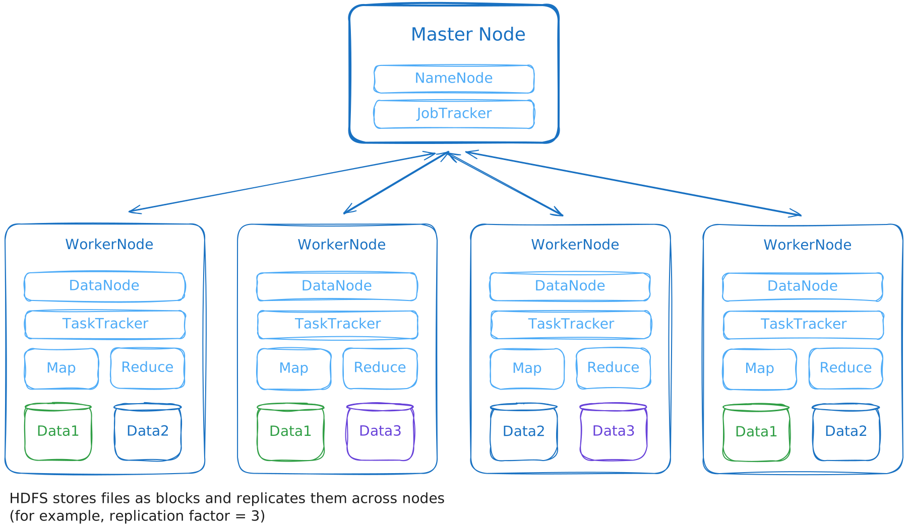
This arrangement tied storage and compute to the same fleet of machines. A team could not add query capacity without also paying for more storage, and could not expand storage without also taking on CPUs that might sit idle. The cluster had to be sized for its busiest hour and kept online around the clock because the data lived on those machines, and turning the cluster off took the data offline with it.
Redshift removed much of that operational work. Instead of buying servers and standing up a cluster, a team could provision a managed, columnar, massively parallel warehouse from the AWS console in minutes.
Queries used SQL over JDBC or ODBC, allowing analysts to connect existing BI tools directly. Hadoop offered SQL layers such as Hive, but these commonly compiled queries into relatively slow MapReduce jobs and often required substantial engineering and cluster administration. Redshift provided a more conventional, interactive warehouse experience without teams having to build and operate that stack.
AWS also handled the rest of the operational burden underneath: node failure, replication, backups, and upgrades. For teams struggling with Hadoop operations, this was a substantial improvement.
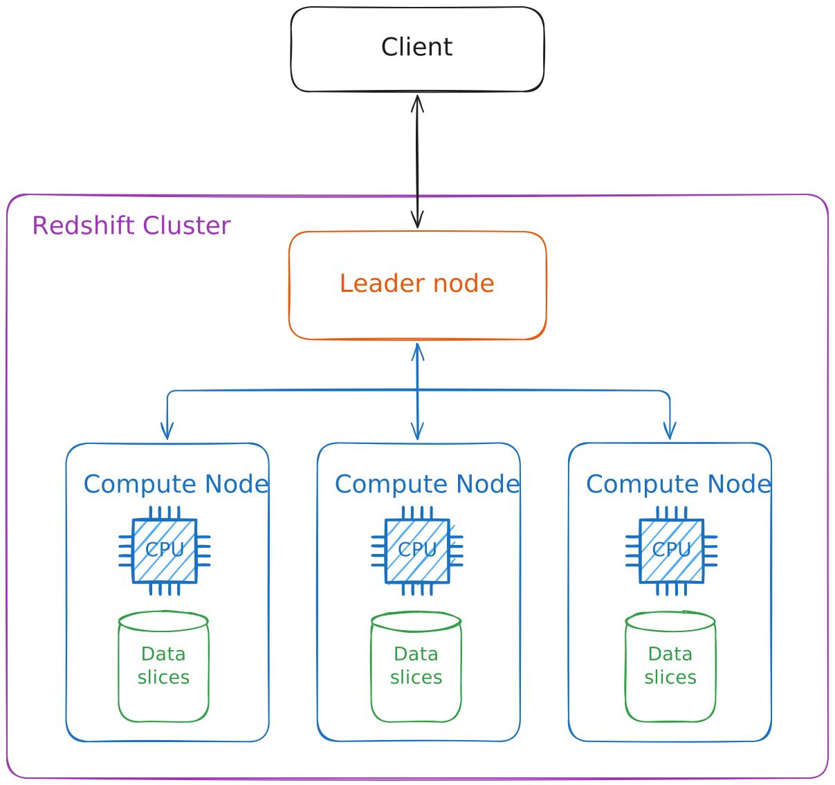
Underneath, though, the machine had the same basic shape as before. Each Redshift node still packed CPU and storage together, and every table was sharded across those nodes. Teams still planned storage and compute capacity together, and resizing meant rebuilding the cluster.
Sharding splits a table's rows across multiple machines so each machine stores and processes only part of the data. Requests are routed to the shard that owns the relevant rows, spreading storage and work across multiple machines.
Physical layout also shaped query performance. Joins ran fastest when matching rows already lived on the same node, so teams chose a distribution key for each table and accepted the tradeoffs that followed. A single cluster still served every workload, with contention managed through workload management queues that defaulted to five queries at a time. Redshift was considerably easier to operate than Hadoop, but the work still had to be organized around the cluster.
Splitting storage and compute
When Snowflake became generally available in 2015, it placed data in object storage rather than on the compute workers. Independent groups of workers would have to fetch the data they needed over the network when a query ran. Hadoop had been designed to avoid exactly this transfer, but by 2015 cloud networks and object storage had become fast and inexpensive enough that data movement no longer had to determine the shape of the entire system.
Reading data over object storage changed both how a warehouse was built and how a team ran one. Because compute no longer had to sit next to the data, capacity stopped being a fixed, up-front commitment and became something you set per job. Spinning up a new warehouse, sizing one up for a heavy load, or sizing it back down afterward was a click, and it took effect in seconds. The capacity planning that had shaped the Hadoop and Redshift years mostly went away.
Competitors spent the following years working toward a similar experience. By 2021, for example, Databricks described its Serverless SQL as starting with cold start latency around 15 seconds, and between 2-6 seconds as of 2026. Redshift also continued to evolve, adding Elastic Resize in 2018, Concurrency Scaling in 2019, and RA3 nodes with managed storage in late 2019. Those changes closed much of the gap, but Snowflake had already become the default answer for data warehousing.
Snowflake's architectural layers
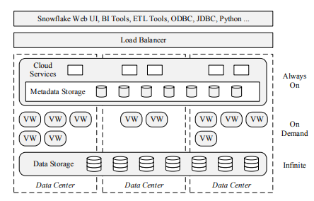
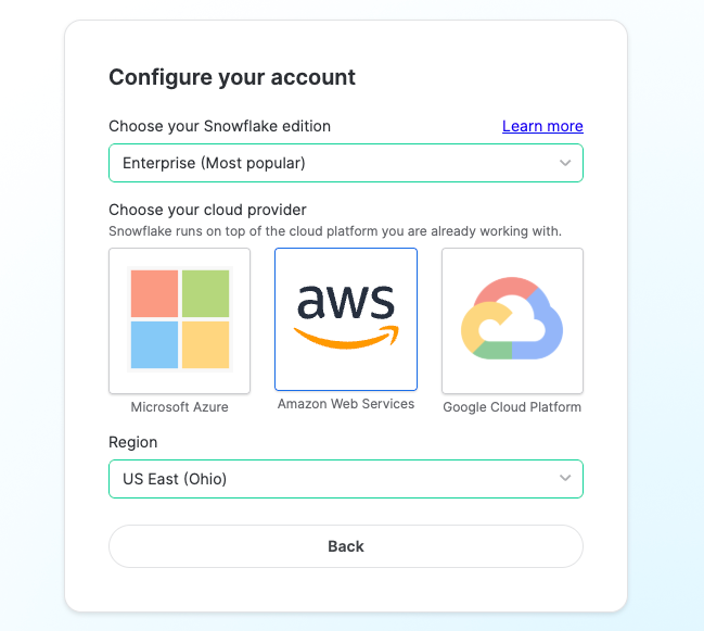
Snowflake's original paper describes three service layers. Compute and cloud services are metered in credits, while storage is billed separately by TB.
Snowflake runs as a managed service on top of the major cloud providers: AWS, GCP, and Azure. The storage layer holds customer data in the chosen provider's object storage, which means S3 when Snowflake runs on AWS. The data is compressed and written in a proprietary columnar format Snowflake calls a micro-partition, with metadata that lets the query engine skip files that a query does not need.
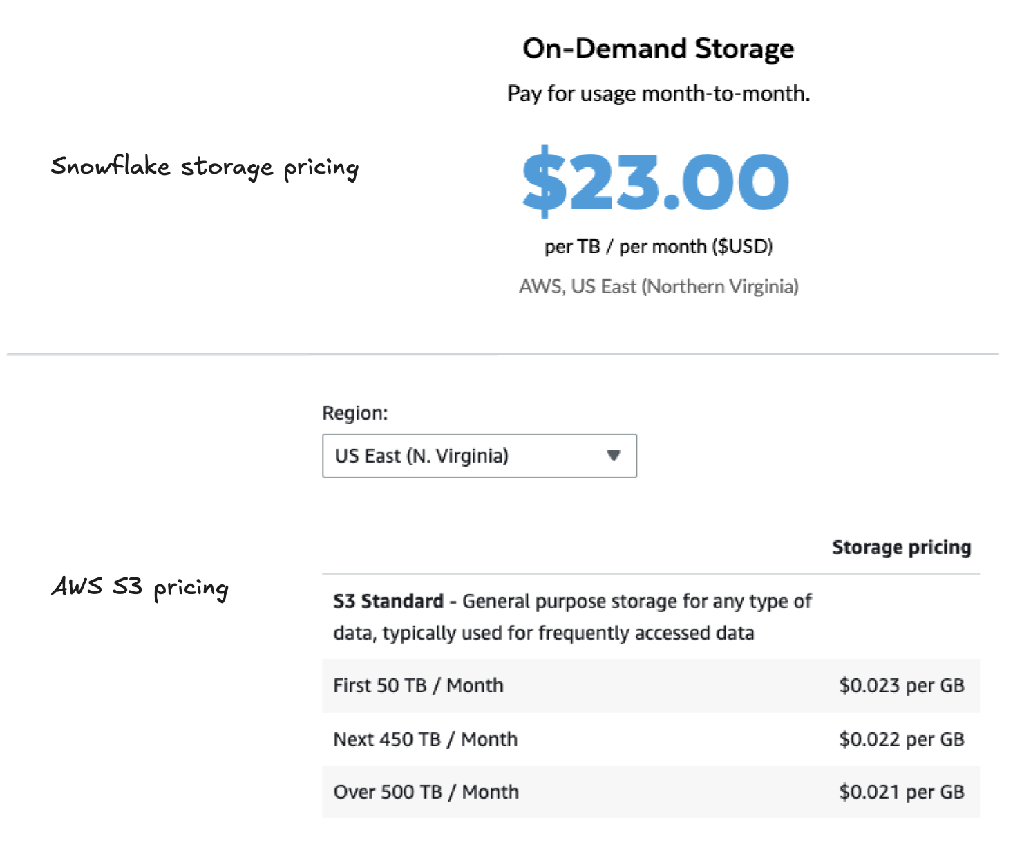
Storage is close to a pass-through of the cloud provider's own price. Snowflake charges about $23 per terabyte per month for on-demand storage in its AWS US regions, which is roughly what S3 costs at low volume. Storage costs are often the smallest part of a Snowflake bill.
A virtual warehouse is the compute that runs your queries. It is a cluster of machines in the cloud, EC2 instances on AWS, running Snowflake's query engine. The warehouse size determines the number of nodes and cost per hour: an X-Small costs 1 credit per hour, a Small costs 2, a Medium costs 4, and the rate doubles at each step. Sizing up mostly means more nodes. The credit count is generally understood to track node count, so a Medium at 4 credits per hour behaves like four nodes' worth of compute.
Cloud services is the metadata and control plane around those warehouses. It is a collection of services that manage virtual warehouses, queries, transactions, authentication, access control, database schemas, and so on. Once storage moved off the workers, that coordination had to live somewhere, so Snowflake runs it as a separate shared layer that lets independent warehouses operate over the same data.
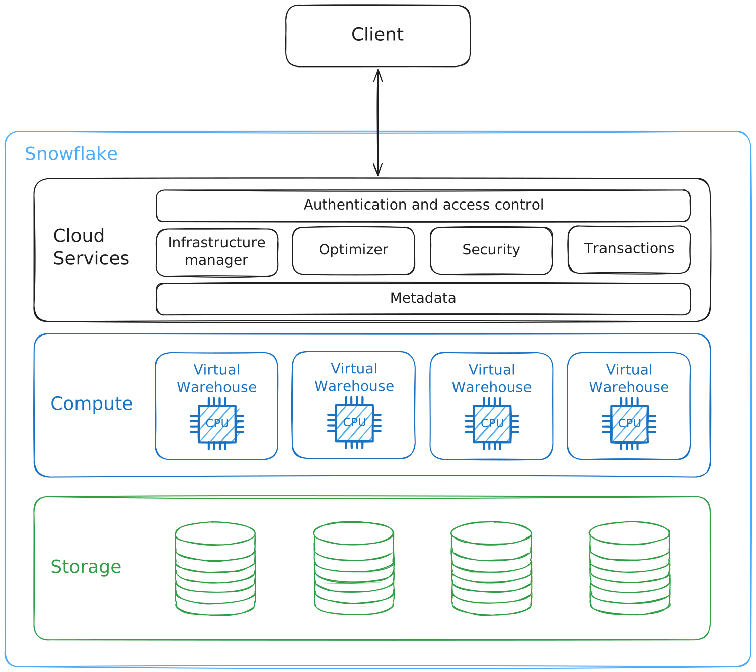
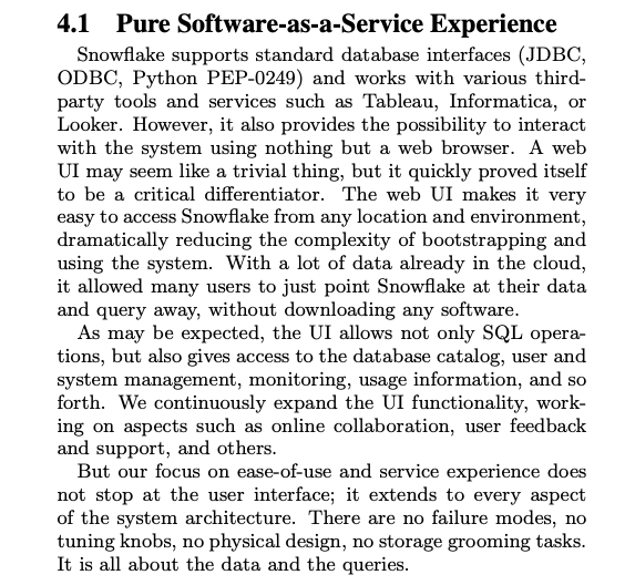
A credit bundles the compute and that coordination into one unit. You choose a warehouse size and spend credits without standing up a metadata service, running control-plane machines, or operating the query engine yourself. That was the goal from the start: Snowflake's founders wanted the warehouse to feel like pure software as a service, where the customer never touches the infrastructure underneath. It also explains why the rented VMs are only one part of what a credit pays for.
From EC2s to Snowflake credits
Snowflake does not publish the machines used by their virtual warehouses, though it is widely accepted that a single X-Small warehouse gets 8 vCPUs and 16 GB of RAM. The community consensus is that Snowflake historically ran on x86 c5d.2xlarge, then moved to Graviton2 for Gen1 and Graviton3 for Gen2.
Since storage costs are largely passed through, the more interesting part of Snowflake's unit economics is the virtual warehouse.
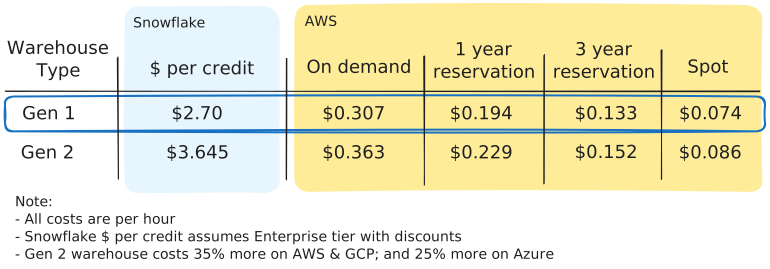
For this estimate, assume the average customer is on Snowflake's Enterprise tier. Enterprise has a list price of roughly $3.00 per credit, but customers purchasing capacity in advance generally receive negotiated discounts. Based on contracts we've seen, a reasonable realized price is $2.70 per credit, with larger customers or those making longer term commitments potentially paying closer to $2.20.
The next step is estimating Snowflake's underlying infrastructure cost.
A standard X-Small warehouse consumes one credit per hour and is generally understood to correspond to one compute node. Each successive warehouse size doubles both the number of nodes and the number of credits consumed. So estimating the economics of one node-hour gives us a rough estimate that can be extended across warehouse sizes.
For a Gen1 warehouse, a c6gd.2xlarge in us-east-1 runs ~$0.307/hr on demand, $0.194/hr on a 1-year reservation, and $0.133/hr on a 3-year reservation. Spot pricing varies, but the most recent price at the time of writing is $0.074/hr.
But Snowflake does not procure infrastructure like an ordinary AWS customer, and the raw on-demand price is not what Snowflake actually pays. Two things pull against each other.
A note on terminology. Snowflake bills in credits and describes warehouses in nodes; AWS sells EC2 instances, and Snowflake's own writing about capacity refers to VMs or servers. Throughout this post I treat one warehouse node as one VM as one EC2 instance as one server.
The free pool
Snowflake maintains what it calls a free pool of pre-provisioned, unassigned virtual machines (VMs) that can be handed to a customer's warehouse on demand. Cloud providers can take up to several minutes to provision new VMs, so Snowflake forecasts demand and keeps ready-to-go instances waiting so that warehouses can resume immediately.
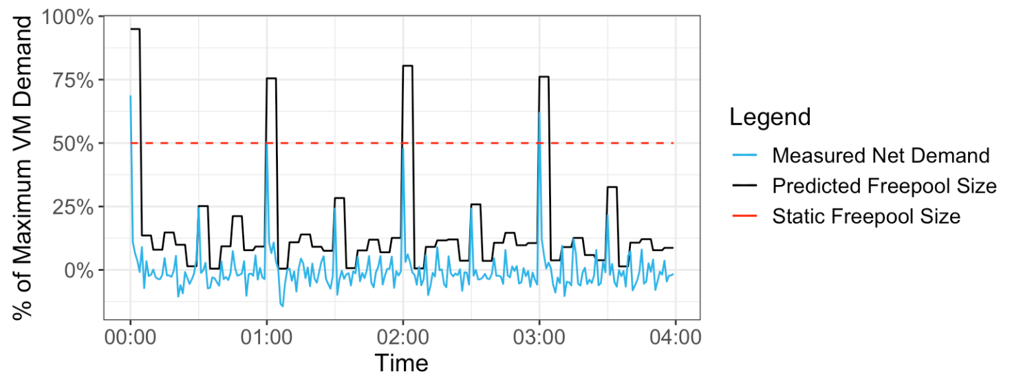
VMs sitting in the free pool are not performing any useful work for customers and represent a cost to Snowflake. So the objective is to minimize free pool server minutes while maintaining their tight internal latency targets for warehouse creation and resumption.
Procurement
At Snowflake's scale, substantial discounts through private pricing agreements and long-term commitments are a given. Snowflake also blends capacity types, optimizing usage with Savings Plans, Reserved Instances, and Spot Instances to hit capacity availability targets.
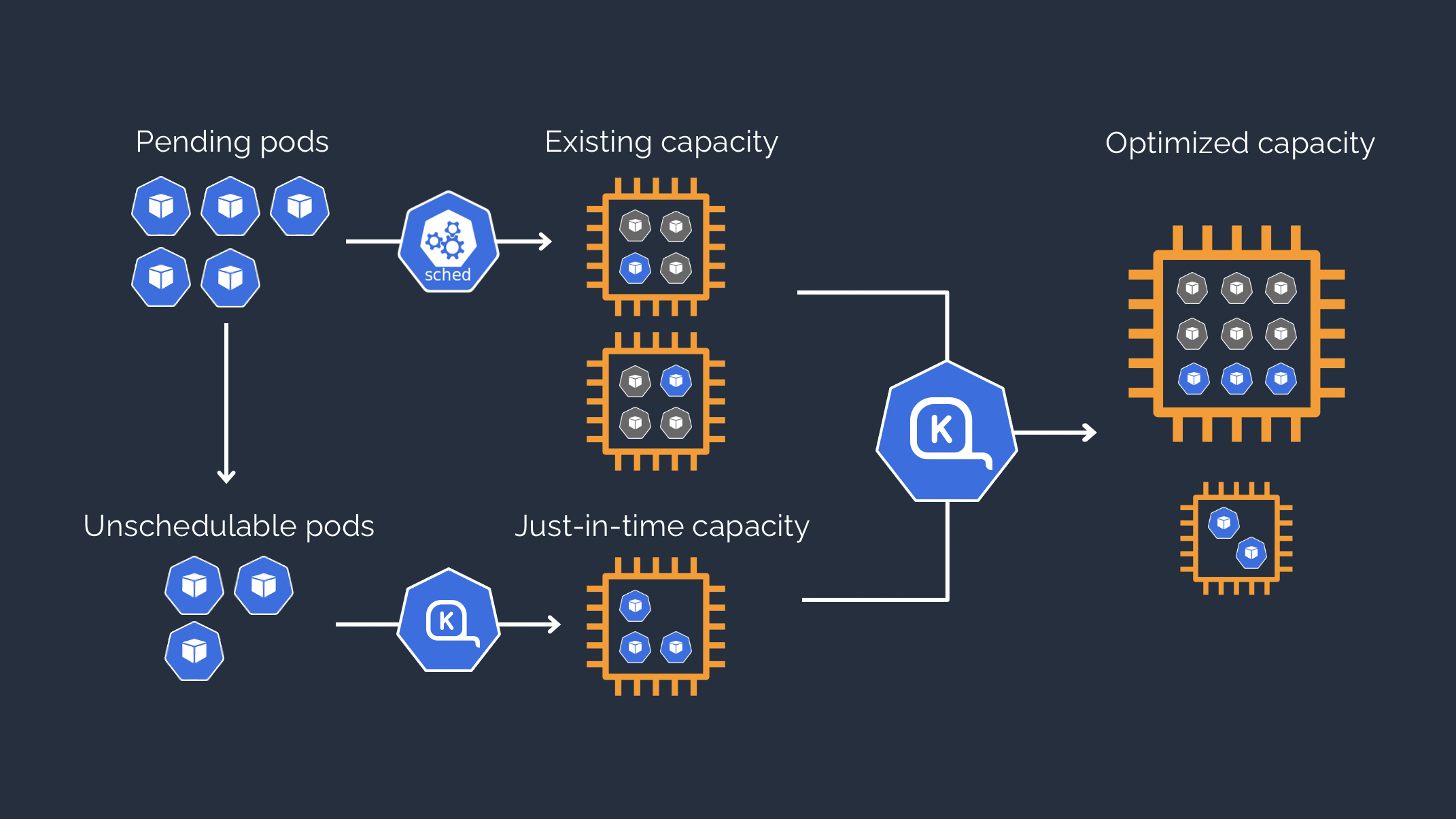
A VP of Engineering at Snowflake confirmed to us that they use Karpenter, which is a Kubernetes autoscaler that provisions both on-demand and spot capacity and handles instance type selection and consolidation dynamically.
Snowflake's margins
Putting it together: one credit buys one node-hour. Assume a 25% private pricing EC2 discount and a 15% free-pool overhead, then compare it against an average $2.70 per credit
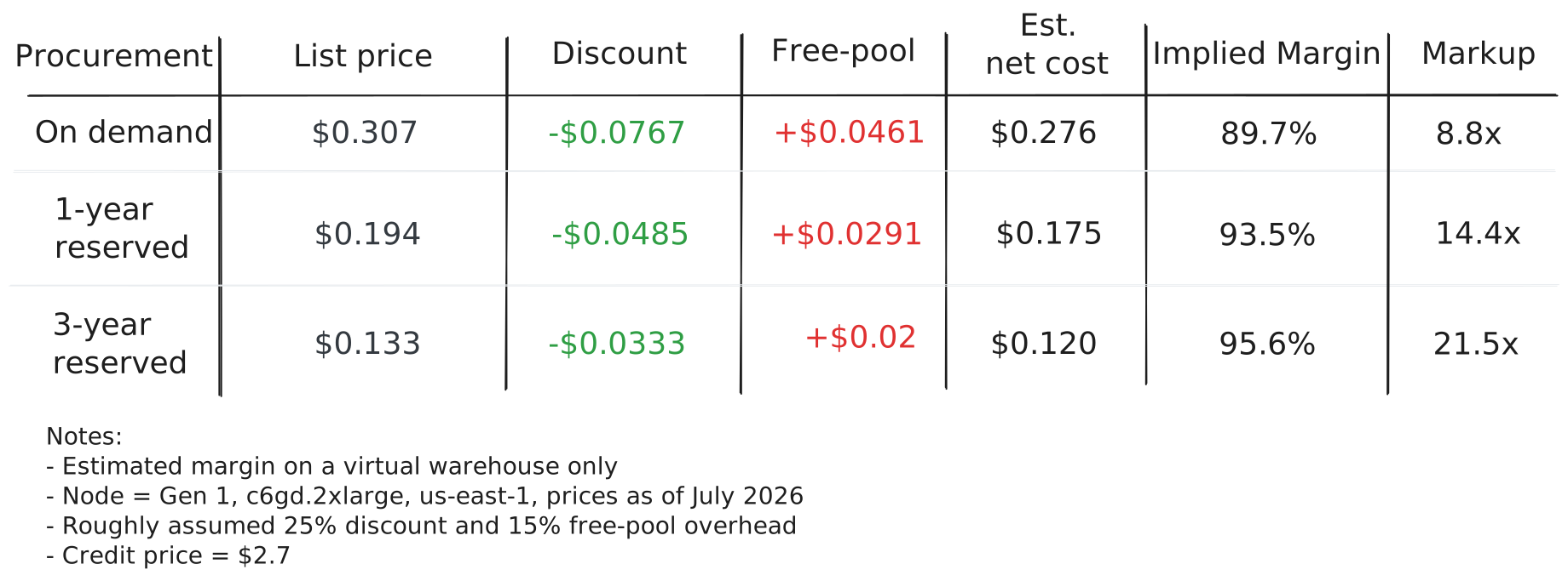
On warehouse compute alone, margin plausibly ranges between 90% up to 96%. If you're using Snowflake purely on running queries, you're roughly paying a 9x premium. Keep in mind this is an estimate. The free-pool overhead and EC2 discount are both guesses, and Snowflake has never published either.
Also keep in mind that this mark up is a narrow slice of the product. Snowflake charges credits for cloud services compute, Snowpipe, automatic clustering, materialized view maintenance, search optimization, Query Acceleration Service, Cortex AI inference, and Snowpark Container Services. None of that is in the table above, and some may run on hardware that costs more than a c6gd.2xlarge.
For reference, Snowflake reported 75.1% product gross margin in Q1 FY2027, so there is clearly something our napkin math doesn't capture.
Why Snowflake commands a premium
A 9x markup is not by itself a problem. Plenty of software carries worse markups, and an EC2 is not the product Snowflake sells. An EC2 does not give you a database. Someone still has to build the query engine, decide how data is laid out, plan work across machines, recover from failures, enforce access controls, and maintain the system as it grows. Snowflake takes that entire burden off the customer.
More importantly, it turns that system into an experience that requires almost no infrastructure management or expertise. A data warehouse once took a team of specialists to provision and maintain. Snowflake bundled much of that work into a managed service operated through a simple web UI that even a non-technical team could manage.
That convenience has economic value. The premium pays for both the managed platform and a significant reduction in organizational complexity.
Convenience can be expensive
Snowflake's premium is easiest to justify when a warehouse is kept busy and sized appropriately for the work it performs. In practice, it's much harder than it sounds.
Snowflake bills for the warehouse that's provisioned, not for the actual work performed. A warehouse may be sized around the largest query it needs to handle even if most of its queries require far less compute. This is especially common in dbt jobs, where conservative sizing can quickly become expensive.
Warehouses can also idle, so teams often spend credits on a warehouse that's not performing any work. Depending on auto-suspend settings, warehouses tend to remain active between queries until the suspension period is met, and each resume carries a minimum billing period. Sporadic usage patterns, like those commonly found in BI and analytics use cases, can keep a warehouse consuming credits even when little to no work is happening.
Concurrency introduces another layer of overhead. When one warehouse is not enough to serve queries, a multi-cluster warehouse adds complete clusters rather than assigning a small amount of incremental capacity. The controls for effectively managing concurrency are limited, with the only options being STANDARD and ECONOMY scaling. A brief concurrency spike may leave customers paying needlessly for excess capacity.

None of this is necessarily a mistake. Snowflake made deliberate tradeoffs in favor of simplicity, elasticity, and predictable performance. The customer doesn't have much to manage, but in exchange, compute is purchased in relatively coarse units that do not always match the shape of the workload.
For much of Snowflake's history, customers had little ability to work around that tradeoff. Snowflake stored the data, governed it, and supplied the engine that processed it. Moving a workload to another engine generally meant moving or duplicating the data and taking on another system to operate.
But that is beginning to change.
True separation of storage and compute
Snowflake separated storage from compute, but only within Snowflake. A customer could create several independent warehouses over the same data, but each warehouse still had to run Snowflake's engine and consume Snowflake credits.
Apache Iceberg takes that separation a step further.
Iceberg changes what a table is. Instead of data living in a proprietary format that only one engine can read, an Iceberg table is a collection of Parquet files in object storage plus metadata describing them, and a catalog that tracks which files make up the current version of a table. Because the table format is not owned by a single warehouse, different engines that implement the Iceberg spec can read the same table.
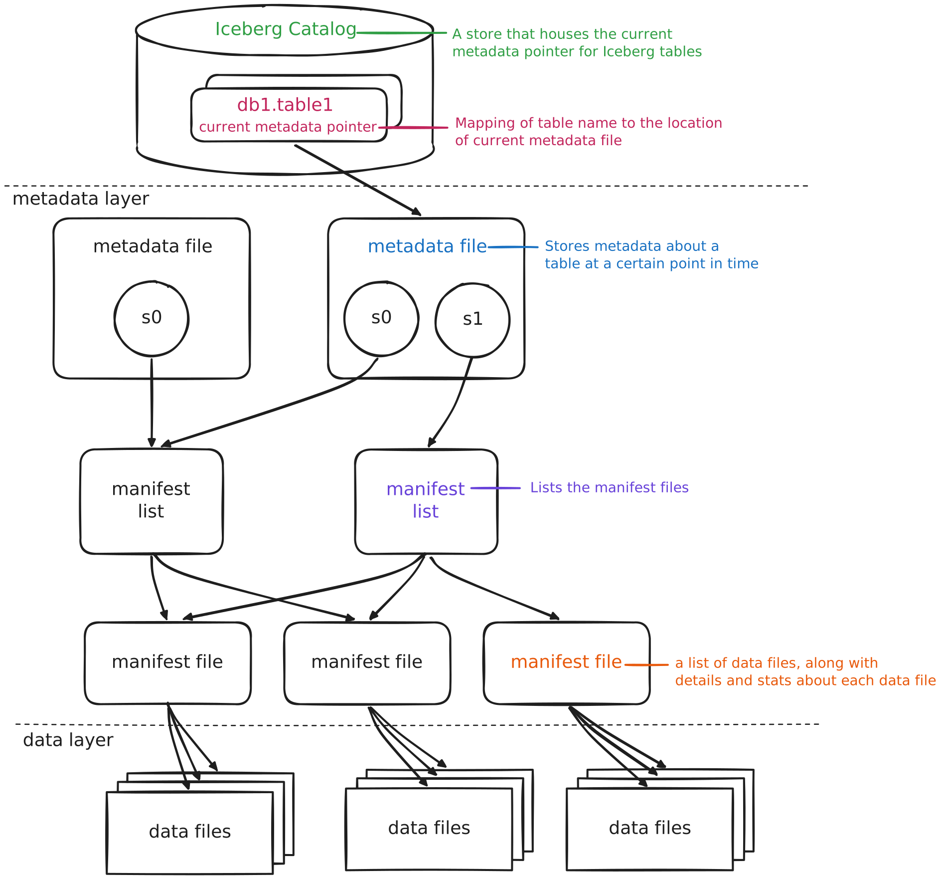
With Iceberg, a customer's data can remain in their own cloud environment while the engine that processes that data can be swapped.
This doesn't mean customers have to replace Snowflake. Snowflake can still catalog the tables, enforce access controls, provide governance, and run the workloads. But those same tables can also be exposed to another compatible engine when a workload has different requirements.
That makes compute a choice rather than a property of where the data is stored, which matters because workloads are not the same shape.
A large nightly transform joining a dozen tables across billions of rows may still belong on Snowflake, and the premium buys something real there. A set of dashboard queries or a smaller transform workload may be better served by a lighter engine running on cheaper machines.
For the first time companies can keep a single governed copy of tables and no longer have to pay the same compute premium every time their data is accessed. They can keep Snowflake as the platform around the data while choosing how individual workloads are actually processed.
Disclosure: this is what we build at Greybeam. We ingest data as Iceberg tables and route eligible queries to DuckDB, falling back to Snowflake when a query is not fit.
Snowflake's tension with shareholders
Iceberg creates an uncomfortable tension for Snowflake. Customers want faster queries, lower bills, and now the freedom to use the best engine for each workload. Snowflake has to support those expectations to remain competitive. Its investments in Iceberg, interoperability, and query performance all make the platform more useful, but they can also reduce credit consumption. Refusing to support Iceberg, though, would've handed the open lakehouse to Databricks.
The difficulty is that Snowflake's revenue is consumption-based. A seat-based company can make its product faster and continue charging the same price. Snowflake can't. When a query runs twice as fast, it consumes fewer credits, and fewer credits mean less revenue for similar work.

That tension eventually surfaced in a class action lawsuit against Snowflake in 2026, which alleged that the company failed to disclose that product efficiency gains, Iceberg Tables, and tiered storage pricing were expected to materially reduce consumption and revenue. The allegations are unproven, but the fact that efficiency gains can become the basis of a lawsuit is a fair description of the position Snowflake is in. It has to make the platform faster, cheaper, and more interoperable to remain competitive, while continuing to grow the consumption its shareholders expect.
That does not mean Snowflake will resist the shift. It means the company has to grow in a different way: by becoming the platform that governs the data and supports more workloads, even when some of the compute happens elsewhere.
The modern data stack moves toward multi-engine
When Snowflake first came to market, a large EC2 instance had a few dozen gigabytes of RAM, object storage was still novel, and the only reasonable way to query against large datasets was to spread them across multiple machines. Distributing work was not a design preference, it was the only thing that worked.
Infrastructure, hardware, and software available today look different. Data processing that used to require the best processors running on large clusters of servers can now run on commodity hardware. EC2s and object storage keep getting cheaper and cheaper, and decades of database research have culminated in free, state-of-the-art query engines like DuckDB, DataFusion, and Polars that can process hundreds of gigabytes of data on a consumer laptop.
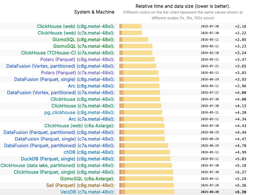
This does not mean that data warehouses are obsolete. Many workloads still scan enormous datasets. Teams still need governance, access controls, and operational simplicity. Snowflake is very good at all of it, but the line between needing a distributed warehouse and running a query on a single machine is starting to blur, and companies have already started acting on it. MotherDuck argues that most analytical data was never big and more than 99% of users never scanned more than a terabyte at once. PostHog rebuilt its data warehouse on DuckDB, giving each organization a single-tenant instance that sleeps when idle. They kept ClickHouse for analytics, where it wins. And they put DuckLake underneath so they aren't locked to DuckDB forever. Cars24 uses StarRocks as a high-speed analytical engine with Snowflake to store long-term, large-volume datasets.
This is also the philosophy behind Greybeam.
We're not trying to replace Snowflake. We are building toward an interoperable, multi-engine data stack where every workload can run on the engine best suited to it.
Greybeam keeps data in Iceberg, routes eligible workloads to DuckDB, and falls back to Snowflake when required. Customers keep the governance and operational experience they already rely on while gaining control over how the compute happens.
Our mission is to make multi-engine analytics practical.