It’s been a while since I wrote the last part in this series, but in working on something else, I accidentally ran into a good candidate for a follow-up with the Miller-Rabin primality test. We’ll explore this algorithm — and as a bonus, if you read this article, you’ll get Pollard’s rho algorithm for factoring — absolutely ☞☞☞ FREE ✪✪✪, operators are standing by, so act now!
Other articles in this series:
- Part 1: Russian Peasant Multiplication
- Part 2: The Single-Pole Low-Pass Filter
- Part 3: Welford's Method (And Friends)
- Part 4: Topological Sort
- Part 5: Quadratic Extremum Interpolation and Chandrupatla's Method
- Part 6: Green’s Theorem and Swept-Area Detection
- Part 7: Continued Fraction Approximation
A funny thing happened to mathematics and physics in the 20th century. Rigid concepts of provability and certainty broke down around 1930, notably with Gödel’s incompleteness theorem and Heisenberg’s uncertainty principle. There are, of course, more everyday notions of incompleteness and uncertainty. I don’t think we’ve grasped these ideas very well in the embedded systems world, and instead of improving our engineering tradeoffs, we’re going down a dangerous road in the name of expediency, understating the consequences of making mistakes. I’ll explain in a roundabout way in this article, through prime numbers and RSA encryption, and in a follow-up article. (This article was originally going to be titled Good, Fast, Cheap: Choose Two, but I decided to save that for another day.)
We’ll start with prime numbers.
Prime Numbers
Suppose you are in need of a large prime number — remember, these are positive integers that cannot be written as a product of two smaller positive integers — because you want to use RSA encryption to communicate securely. Or maybe you just collect prime numbers, and you want one to tattoo on your arm. Whatever.
So you generate some large odd random numbers which are candidates, and you want to check to see if they are prime. This isn’t a wild goose chase: the Prime Number Theorem says that for large \( N \), the prime-counting function \( \pi(N) = \) the number of primes less than \( N \), is approximately \( N / \ln N \), asymptotically approaching it as N gets larger. Prime numbers aren’t actually that rare; the density of prime numbers around \( N \) is approximately \( 1 / \ln N \). This means that for M-bit numbers (that are on the order of \( N=2^M \)), approximately one out of every \( \frac{1}{2} M \ln 2 \) odd values is prime, so on average roughly one out of every 11 odd 32-bit numbers is prime, one out of every 22 odd 64-bit numbers is prime, one out of every 44 odd 128-bit numbers is prime, and so on.
You might say: well, that’s just the average distance between prime numbers; surely there are bunches where they are more common, and “deserts” where they are less common. This is an area of obsessive study among a subset of very respectable mathematicians, who have defined the “prime gap” \( g_n = p_{n+1} - p_n \) as the difference between successive prime numbers; indeed, there was a recent improvement in 2014 on a lower bound on this gap, proving that
$$\max_{p_{n+1} \leq X} (p_{n+1}-p_n) \gg \frac{\log X \log \log X\log\log\log\log X}{\log \log \log X},$$
which is oddly mesmerizing, something like a mathematical analogloglogue of the phrase “How much wood could a woodchuck chuck if a woodchuck could chuck wood?” They — the subset of very respectable mathematicians — have also defined a ratio called the “merit” of prime gaps, which is the ratio \( M = g_n / \ln p_n \) — basically how much larger the actual gap \( g_n \) is than the average gap \( \ln p_n \) — and so far, the largest known merit \( M \) has topped out at just under 42: the 288-bit number \( p_n = \) 293703234068022590158723766104419463425709075574811762098588798217895728858676728143227 has a gap \( g_n = 8350 \) between it and its next-higher prime neighbor. So for 288-bit numbers, you might have to check half of the worst-case gap \( g_n = 8350 \) — in other words, 4175 different odd 288-bit numbers — instead of the average gap of 100 odd numbers. Even 4175 isn’t a very large set of numbers to check.
(A list of prime gaps was maintained for about 20 years by a Dr. Nicely, now sadly deceased, who also discovered the Pentium division bug while running calculations in his number theory research. In this list of prime gaps, the record merit for 41.9388… was found as a result of the “Gapcoin” cryptocurrency project in 2017. I do not partake in or endorse cryptocurrency, but you have to admit it’s a nifty idea to produce mathematical research data as a side effect of crypto mining.)
So again, finding a prime near a given value isn’t a wild goose chase.
Once you have a candidate number, you have to see if it is prime, and there are various methods for doing this.
Trial division
The grade-school approach is called trial division, which checks for prime divisors up to the square root of \( N \), at which point if you have not found a divisor then \( N \) is prime. (If \( N \) is odd then you only have to check the odd prime divisors.)
Suppose my two candidates are 1961 and 1973. The square root of 2000 is 44.72…, so it’s a matter of checking all the prime divisors between 3 and 43, which are 3, 5, 7, 11, 13, 17, 19, 23, 29, 31, 37, 41, and 43 (13 divisors), or if I don’t want to keep track of which numbers are prime, I just divide by all the odd numbers between 3 and 43 (21 divisors).
If we do this, we find that 1961 = 37 × 53, and there are no divisors of 1973 which are less than 44, so 1973 is prime.
Hurray!
This approach was documented by Leonardo of Pisa — aka Fibonacci — in his 1202 manuscript Liber Abaci. (In case you’re like me and can’t read medieval Latin, but are curious, see the Addenda.)

The number of steps it takes is roughly proportional to the square root of \( N \) — in Big O notation, this is \( O(\sqrt{N}) \).
Differences of squares
The next development in prime factorization, according to Richard Mollin’s A Brief History of Factoring and Primality Testing B. C. (Before Computers), was Pierre de Fermat’s differences of squares method, which finds factors of \( N \) when they are reasonably close to the square root, by looking for some positive integer \( a \) where \( a^2 - N = b^2 \), in which case we can write \( N = a^2 - b^2 = (a+b)(a-b) \).
For example, with \( N=1961 \), we start with \( a=45 \) and immediately get \( 45^2 - 1961 = 64 = 8^2 \), yielding \( 1961 = (45 + 8)(45 - 8) = 53 \times 37. \)
Other numbers take a little longer; for example with \( N = 1943 = 29 \times 67 \), we have:
- \( 45^2 - 1943 = 82 \)
- \( 46^2 - 1943 = 173 \)
- \( 47^2 - 1943 = 266 \)
- \( 48^2 - 1943 = 361 = 19^2 \to 1943 = (48 - 19)(48 + 19) = 29 \times 67. \)
Residues
Fermat also came up with a method using congruences (modular arithmetic), known as Fermat’s little theorem:
If \( p \) is a prime number, then for any integer \( a \), then \( a^p \equiv a \pmod p \).
The modular arithmetic isn’t difficult; you just engage in repeated squaring and multiplication, also known as Russian Peasant Multiplication. For example, suppose we want to look at \( p=1283 = \) 1024 + 256 + 2 + 1, and we pick \( a = 8 \):
- \( a^2 \pmod p \equiv 8 \times 8 \equiv 64 \)
- \( a^4 \pmod p \equiv 64 \times 64 \equiv 247 \pmod p \)
- \( a^8 \pmod p \equiv 247 \times 247 \equiv 708 \pmod p \)
- \( a^{16} \pmod p \equiv 708 \times 708 \equiv 894 \pmod p \)
- \( a^{32} \pmod p \equiv 894 \times 894 \equiv 1210 \pmod p \)
- \( a^{64} \pmod p \equiv 1210 \times 1210 \equiv 197 \pmod p \)
- \( a^{128} \pmod p \equiv 197 \times 197 \equiv 319 \pmod p \)
- \( a^{256} \pmod p \equiv 319 \times 319 \equiv 404 \pmod p \)
- \( a^{512} \pmod p \equiv 404 \times 404 \equiv 275 \pmod p \)
- \( a^{1024} \pmod p \equiv 275 \times 275 \equiv 1211 \pmod p \)
- \( a^{1280} = a^{1024}a^{256}\pmod p \equiv 1211 \times 404 \equiv 421 \pmod p \)
- \( a^{1282} = a^{1280}a^2\pmod p \equiv 421 \times 64 \equiv 1 \pmod p \)
- \( a^{1283} = a^{1282}a\pmod p \equiv 1 \times 8 \equiv 8 \pmod p \)
Leonhard Euler proved Fermat’s little theorem in 1736. (Fermat had a habit of stating theorems without proof.) This theorem happens to be a consequence of some properties of group theory; as I stated in Part 1 of my Linear Feedback Shift Registers for the Uninitiated series:
Fermat’s little theorem that \( a^p \equiv a \pmod p \) is an immediate consequence of the structure of the cyclic group \( \mathbb{Z}_p{}^* \): you can take any element \( a \) of the group and it will always form cycles that divide the group order \( p-1 \), so \( a = a^1 \equiv a^{1 + k(p-1)} \pmod p \) for any \( k \), and Fermat’s little theorem is just the case where \( k=1 \).
Fermat’s little theorem also implies, through contraposition, that if you have a number \( N \) and can find an integer \( a \) such that \( a^N \not\equiv a \pmod N \), then \( N \) is not prime.
def test_fermat_little(a, N):
    """
    Computes a^N mod N
    """
    return pow(a,N,N)

test_fermat_little(8, 1283)
test_fermat_little(8, 1961) # Aha! 1961 is not prime!
Unfortunately, the converse of Fermat’s little theorem is not true; there are composite integers \( N \) called Carmichael numbers or Fermat pseudoprimes, that satisfy \( a^N \equiv a \pmod N \) for all \( a \). These are like “impostor primes”, and the first one is 561 = 3 × 11 × 17:
for a in range(2, 20):
    print(a, test_fermat_little(a, 561))
2 2
3 3
4 4
5 5
6 6
7 7
8 8
9 9
10 10
11 11
12 12
13 13
14 14
15 15
16 16
17 17
18 18
19 19
So while Fermat’s little theorem can definitely prove that some numbers are not prime, numbers that pass this test are either prime numbers or Carmichael numbers.
The quirk in Fermat’s test is that while it can be used to show a number is composite, it gives no information about the factors of that number: knowing that a number is prime is a weaker result than knowing its factors. At this time of writing, \( 2^{1277}-1 \) is the smallest Mersenne number (= numbers of the form \( 2^M-1 \)) that is known to be composite, but hasn’t been factored yet, despite our advances in computation and in factoring algorithms. But Fermat’s test is lightning-fast to demonstrate that \( 2^{1277}-1 \) is a composite number:
M1277 = (1 << 1277) - 1
test_fermat_little(3, M1277)    # Not a prime, otherwise the result would be 3
39029102728836828830242049046976630362068695324460194418075965880583048150375624
36669737990935338176087285415361828868532938827618069620197571187624752921741603
50019728641505765874636099442964764645852582671788018607038915575957923661045781
97171303979907409066229476609046670110804713165497444097326431457784202122005345
1471922636509411814268315629153968481818318060901542276483137223
In the years since Fermat and Euler, there have been various advances in methods to test for primality and to factor numbers.
Nondeterministic methods
The 1970s were an interesting decade in number theory — all of a sudden, mathematicians seemed to be interested in primality testing and factoring.
Computers had been around for over 20 years, but it took until about 1969 for a majority of universities in the USA to have a computer on campus; in 1965 only about a third of U.S. universities had computers. The number of computers in the 1950s and early 1960s was much smaller, but rapidly increasing; thirty universities in the southeast US alone had computers in 1961. And maybe it took a while for programming to diffuse through the various departments to become more normalized.
Carl Pomerance stated this about the mathematics community in his 1996 article, A Tale of Two Sieves:
In the middle part of this century, computational issues seemed to be out of fashion. In most books the problem of factoring big numbers was largely ignored, since it was considered trivial. After all, it was doable in principle, so what else was there to discuss? A few researchers ignored the fashions of the time and continued to try to find fast ways to factor. To these few it was a basic and fundamental problem, one that should not be shunted to the side.
In other words: factoring wasn’t cool. And yet the “few researchers” such as Daniel Shanks, John Pollard, Derrick and Emma Lehmer, R. Sherman Lehman, Richard K. Guy, and Gary Miller were exploring newer and faster algorithms for prime factorization and testing.
For instance, Pollard published a Monte Carlo Method for Factorization in 1975, now known as the rho method, which has expected runtime of \( O(\sqrt[4]{N}) \) — much faster than the trial division approach. (If this sounds vaguely familiar, perhaps it’s because I’ve mentioned the rho method for discrete logarithms in Part Five of my series on linear-feedback shift registers. Same general idea but different computational problem: try different values generated by repeated iterations of a function, until you find a cycle. We’ll cover Pollard’s rho algorithm for factoring in just a minute.)
Monte Carlo methods and algorithms
The term Monte Carlo in algorithms refers to a random or nondeterministic or stochastic algorithm — you don’t necessarily know how long it’s going to take, or even how accurate the answer is in some cases.
These algorithms were pioneered during the Second World War for certain applied physics calculations, such as multidimensional numerical integration, and the general idea is to take enough samples from a statistical ensemble that the set of samples models the ensemble with sufficient accuracy.
Some examples may make this concept clearer, and show different types of Monte Carlo methods:
- determining an unknown probability distribution (example: tolerance analysis)
- determining aggregate statistics over a distribution (example: numerical integration)
- finding solutions (example: Pollard’s rho algorithm)
- probabilistic proofs (example: Miller-Rabin test)
Tolerance analysis and coin-flipping
The method you will probably run into most as an electrical engineer is Monte Carlo simulation of tolerance analysis. Even a simple resistor divider involves a nonlinear equation:

The exact probability distribution of \( \alpha = \frac{R_2}{R_1+R_2} \), if resistances \( R_1 \) and \( R_2 \) are normal distributions, does not have a closed-form solution because of the nonlinearity. But you can approximate the result if the variances are small; alternatively you can just simulate a million different random samples of \( R_1 \) and \( R_2 \) and approximate the distribution of the divider ratio \( \alpha \) numerically:
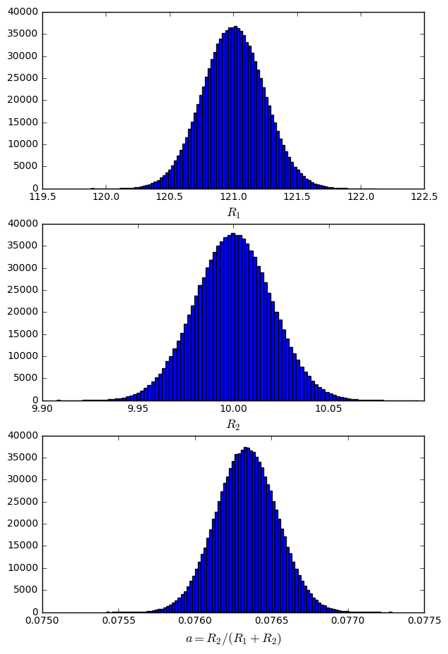
This example is from another article I wrote on tolerance analysis, and the statistical summary of \( \alpha \) in this case (\( R_1 = \) 121 kΩ, \( R_2 = \) 10 kΩ, both with a standard deviation of 0.2%) is \( \alpha \approx \) 0.07634 with a standard deviation of \( \sigma_\alpha \approx \) 0.00020, and a range over the million trials of between 0.07542 and 0.07729.
If you really want to get into the statistics, it’s possible to analyze bounds on the experimental results itself: the exact value of \( \alpha \) for nominal values of the resistors is simply \( \alpha = \frac{10}{10+121} = \frac{10}{131} \approx \) 0.076336, and in that article I didn’t use enough digits to represent the numerically-calculated mean value to see how far away it was from the expected value.
The point is that for any numerical result of a Monte Carlo simulation, there’s an expected and worst-case bound on the error for a given number of iterations or function evaluations. For 100 iterations of Monte Carlo analysis, you might get the result within 0.01% worst-case, and within 0.0001% (one part per million) on average, but it’s likely that the chances of being anywhere near worst-case are extremely small.
Another example: suppose we have some object, and need to measure the likelihood of something happening, like radioactive decay of a lump of uranium, or the chances of an unfair coin coming up heads. In the case of a coin, suppose the coin has a 25% chance of coming up heads and a 75% chance of coming up tails, but we don’t know that. How many heads are we likely to get? Well, worst case we could see zero or 400, but it’s insanely unlikely to get those extreme results:
import numpy as np
import scipy.stats
import pandas as pd
from IPython.core.display import HTML

p = 0.25            # probability of heads

flips = np.arange(30,201,10)
# hypothetical number of heads

nflips = 400
cdf = scipy.stats.binom.cdf(flips, nflips, p)
sf = scipy.stats.binom.sf(flips, nflips, p)

##### the rest of the code below is just for formatting #####

def regroup(x):
    return (x.cdf,x.sf)
df = pd.DataFrame({'# heads':flips})
df['CDF'] = pd.DataFrame(dict(cdf=cdf, sf=sf)).apply(regroup, axis=1)

def format_cell(x):
    cdf, sf = x
    if cdf > 0.9999:
        return '1 - %.5lg' % sf
    elif cdf < 0.00001:
        return '%.5lg' % cdf
    else:
        return '%.9f' % cdf
(df.style
   .map(lambda cell: 'text-align: right')
   .format({'CDF':format_cell})
   .hide(axis="index")
)
| # heads | CDF |
|---|---|
| 30 | 9.6332e-20 |
| 40 | 2.5517e-14 |
| 50 | 4.3326e-10 |
| 60 | 7.8008e-07 |
| 70 | 0.000209414 |
| 80 | 0.010846896 |
| 90 | 0.135845909 |
| 100 | 0.526837586 |
| 110 | 0.886537193 |
| 120 | 0.990029782 |
| 130 | 0.999695770 |
| 140 | 1 - 3.2118e-06 |
| 150 | 1 - 1.1883e-08 |
| 160 | 1 - 1.5665e-11 |
| 170 | 1 - 7.4719e-15 |
| 180 | 1 - 1.3057e-18 |
| 190 | 1 - 8.4307e-23 |
| 200 | 1 - 2.0206e-27 |
The second column shown above is the cumulative distribution function (CDF), which is the probability that the number of heads will be less than or equal to any particular value. For 400 coin flips with \( p = \) 0.25 for heads, the number of heads is going to be between 70 and 130 about 99.95% of the time (= 0.9997 − 0.0002). The chances of being below 40 or above 170 are less than one in a trillion. And if you want less uncertainty, just run more trials. You can make the error arbitrarily low, depending on how much work you want to do.
The output of both of these examples (resistor tolerance, number of coin flips) are distributions, where we run an experiment some number of times to see how the result varies.
Monte Carlo integration
The second type of Monte Carlo algorithm is one where the target is an aggregate measurement rather than a probability distribution. For example, Monte Carlo integration, which I covered in a recent article, approximates the infinite sum of integration, by a finite sum at random points scattered throughout some boundary. Here are 20000 points within the unit square \( (x,y) \) where 15654 (78.27%) of them are within the circle \( x^2 + y^2 = 1 \) and therefore the circle area is approximately \( 4\cdot\frac{15654}{20000} = 3.1308. \)

There are easier and more accurate ways to integrate the area of a circle numerically, but in multidimensional integration, Monte Carlo integration is more competitive with other techniques.
Birthday attack! (Pollard’s rho algorithm)
The two Monte Carlo methods we’ve discussed so far are used for making numerical estimates, where using more samples increases the accuracy of the estimate. The end goal of the estimates are to approximate real-world quantities: areas, volumes, definite integrals, probability distributions.
Other methods have different goals. Pollard’s rho algorithm, for example, is a probabilistic approach to factoring integers, where the randomness avoids any correlation with the number-theoretical structure of integers less than some candidate \( N \).
Instead of trying directly to find some factor \( d \) that divides \( N \), Pollard’s method tries to find two values \( x_j \) and \( x_k \) such that \( d = \gcd(x_j - x_k, N) \ne 1 \), and \( d \ne N \). As soon as such a \( d \) is located, we have found a nontrivial divisor of \( N \), and then can reduce the problem of finding the prime factors of \( N \) to finding the prime factors of \( d \) and \( N/d \). The values \( x_j \) and \( x_k \) are iterative evaluations of a polynomial \( f(x) \) with integer coefficients, such as \( f(x) = x^2 + a \): suppose \( x_0 \) is a random integer between 0 and \( N-1 \); then \( x_1 = f(x_0) \pmod N \), and in general \( x_j = f(x_{j-1}) \pmod N \). The values \( x_j \) and \( x_k = x_{2j} \) are the “tortoise” and the “hare” where the “hare” iterates function \( f(x) \) twice for each iteration of the “tortoise”.
The bigger question with this algorithm: why does it work?
Imagine a really large room with people, each of which represents an integer between 1 and \( N-1 \), and we’re going to label them each with their value modulo some smaller number \( d \). Imagine for a moment that \( d=365 \) and therefore the label corresponds to each person’s birthday: 0 = January 1, 1 = January 2, and so on, all the way to 364 = December 31. (Leap year babies have been excluded for the purpose of this thought experiment.) One question is how many people do you need to gather before you find two with the same birthday? The answer depends on luck, but tends to be around 20-30 people because of the birthday paradox — the second person has a 1/365 chance to match the first person’s birthday, but if there isn’t a match, then the third person has a 2/365 chance to match either of the first two people’s birthdays, and if there still isn’t a match, then the fourth person has a 3/365 chance to match any of the first three people’s birthdays, and so on. It is theoretically possible that 365 people are in a room and none of them have the same birthday, but this is astronomically unlikely if they are chosen at random. Even 90 people in a room make it very likely that at least two of them will have the same birthday; the probability that their birthdays are all different is about one in 163,000:
$$\begin{aligned} p_{90|365} &= \prod\limits_{k=0}^{89} \frac{365-k}{365} \\ &= \frac{365}{365}\times\frac{364}{365}\times\frac{363}{365}\times\frac{362}{365}\times \; \ldots \times \frac{276}{365} \\ &= \frac{365!}{(365-90)! \times 365^{90}} \\ &\approx 6.15 \times 10^{-6} \end{aligned}$$
The expected number of people before you get a match is roughly proportional to the square root of \( d \). Now instead of \( d = 365 \), imagine that \( p_1 \) is the smallest factor of \( N \). You only need to gather around \( \sqrt{p_1} \) different values before you find two that have the same remainder modulo \( p_1 \). If you take Pollard’s approach, you don’t even need to know \( p_1 \) — which is the whole point! — and finding two values \( x_j \) and \( x_k \) with the same remainder modulo \( p_1 \), will result in \( \gcd(x_j - x_k, N) = mp_1 \), a multiple of \( p_1 \), thus revealing some factor of \( N \). Pollard’s method magically does the same thing without actually “gathering” the different values. The magic comes from the fact that the polynomials \( f(x) \) with integer coefficients behave identically modulo \( N \) and modulo any positive integer \( d \) that is a divisor of N — in other words, \( f(x) \mod N \mod d = f(x) \mod d \) — and as soon as there’s a repeated value modulo \( d \), all future values modulo \( d \) repeat in a cycle. This is easier to see with an example, so here’s Pollard’s algorithm finding a factor of \( N = 286827707 = 1229 \times 419 \times 557 \):
import math

def factor_pollard_rho(n,
                       watcher=None,
                       extra_iterations=0):
    def f(x):
        return (x*x + 1) % n
    def dummy(x):
        pass
    if watcher is None:
        watcher = dummy

    # Five trials; these are just some different starting values
    for start in [2, 3, 7, 11, 13]:
        tortoise = start
        hare = start
        # just in case we want to examine the intermediate values
        watcher(hare)
        d = 1
        while d == 1:

            tortoise = f(tortoise)
            prevhare = f(hare)
            hare = f(prevhare)

            # just in case we want to examine the intermediate values
            watcher(prevhare)
            watcher(hare)
            d = math.gcd(abs(tortoise - hare), n)


        if d == n:
            continue
        else:
            e = n//d
            if d*e != n:
                raise ValueError("Hmm we have a problem")

            # keep going only for illustrative purposes
            x = hare
            for _ in range(extra_iterations):
                x = f(x)
                watcher(x)
            return d, e

    return None

def make_watcher(dlist):
    widths = [math.ceil(math.log10(d)) for d in dlist]
    def row(xlist):
        return(' '.join('%*d' % (w,x) for w,x in zip(widths, xlist)))
    header = ' j '+row(dlist)
    j = [0]
    print('    x_j mod')
    print(header)
    print('-'*len(header))
    def watcher(x):
        print('%2d ' % j[0] + row(x%d for d in dlist))
        j[0] += 1
    return watcher

p1,p2,p3 = (1229,419,557)
N=p1*p2*p3
factor_pollard_rho(N, watcher=make_watcher([N,p1,p2,p3,233383]),
                   extra_iterations=6)
    x_j mod
 j 286827707 1229 419 557 233383
--------------------------------
 0         2    2   2   2      2
 1         5    5   5   5      5
 2        26   26  26  26     26
 3       677  677 258 120    677
 4    458330 1142 363 476 224947
 5 108507377  196 204 435 217665
 6   3870439  318 136 403 136311
 7 147399233  347  61 323 134560
 8 237190823 1197 370 171  73695
 9  80180985 1025 307 278 130616
10 285202800 1060 394 419   8774
11  73715715  295 207 107 200070
12  84271068  996 112 310  19805
13  98642212  214 394 297 154586
14 221526345  324 207 204  45878
15  72258338  512 112 399 142991
16 106630866  368 394 457 208218
17 148307352  235 207 532 109147
18  14502121 1150 112  69  32375
19 260239618   97 394 306  17573
20  10546856  807 207  61  44621
21  84294532 1109 112 380  43269
22 254628789  882 394 138   7936
23  22371455 1197 207 107 200070
24  61632917 1025 112 310  19805
25 239372161 1060 394 297 154586
26 244164496  295 207 204  45878
27  30716164  996 112 399 142991
28 276300307  214 394 457 208218
29 227190806  324 207 532 109147
30 225713736  512 112  69  32375
You can see the loops in each of the prime divisors — as soon as there’s a repeated value of \( x_j = x_{j+L} \pmod d \) for any divisor \( d \), then because each \( x_{j+1} \mod d = f(x_{j}) \mod d \) is a deterministic function of the previous value, all future values will repeat in loops, and the cycle-finding algorithm will catch it and identify some divisor \( d \). For \( d=1229 \), the loop length is 15; for \( d=419 \), the loop length is 3; and for \( d=557 \) the loop length is 12. It might be theoretically possible for all prime factors \( p \) to not reach a loop until \( j=p \) instead of \( \sqrt{p} \), but this is, like the birthday paradox, extremely unlikely.
So even though it’s not clear how long it will take to find a factor — there’s the uncertainty — eventually Pollard’s algorithm will find a factor, and once it does, it is easy to verify, so you’re done: the uncertainty is gone.
The Miller-Rabin test
Other types of nondeterministic algorithms are a little bit weirder, more like the coin flip example, where the probability never actually hits zero but can be reduced below arbitrary bounds. Primality testing is one of these cases. In the 1970s, a few mathematicians in the area of number theory were exploring nondeterministic algorithms for primality testing; the two classic methods are the Solovay-Strassen test (submitted for publication in 1974, published in 1977) and the Miller-Rabin test (Gary Miller’s deterministic version in 1975, with Michael Rabin’s fast nondeterministic versions in 1976 and 1977, published in 1980).
Miller-Rabin is easier to understand than Solovay-Strassen, and is still widely used today. Here’s how it works:
- Suppose your number is \( N \). (We’ll just use \( N=1961 \) again as an example.)
- You figure out \( s \), the largest power of two that divides \( N-1 \), writing it as \( N-1 = 2^sd \). (\( 1960 = 2^3 \times 245 \), so \( s=3 \) and \( d=245 \).)
- Then you run some number of iterations of the following test, each time choosing a random number \( a < N \), called a “base”. There are three distinct results that can occur on each iteration:
- The test failed: base \( a \) has a common factor with \( N \), in which case \( N \) is composite, and we can stop. Game over. This is easy to check with the Euclidean GCD algorithm.
- The test failed: base \( a \) is a “witness” that proves \( N \) is composite, using a modular arithmetic calculation (see below)
- The test passed: base \( a \) is not a witness, in which case \( N \) is “possibly prime”. (The technical phrase is \( N \) is a strong probable prime to base \( a \))
For each iteration of the Miller-Rabin test:
- If \( \gcd(a,N) \ne 1 \), then \( N \) is composite: stop; the test failed.
- Define \( y[k] = a^{2^kd} \pmod N \), so that \( y[0] = a^d \pmod N \) and \( y[k+1] = (y[k])^2 \pmod N \)
- If \( y[0] = a^d \equiv 1 \pmod N \), this implies that \( y[s] = a^{N-1} \equiv 1 \pmod N \) (Fermat’s little theorem) and \( N \) is “possibly prime” (\( a \) is not a witness). The test passed.
- Otherwise, for each \( k = 0, 1, … s-1 \):
- if \( y[k] \equiv -1 \pmod N \), this also implies that \( y[s] = a^{N-1} \equiv 1 \pmod N \) (Fermat’s little theorem), and \( N \) is “possibly prime” (\( a \) is not a witness), in which case we can stop. The test passed.
- Otherwise, we know \( y[k] \not\equiv \pm 1 \pmod N \). Compute \( y[k+1] = (y[k])^2 \pmod N \), and if it is 1, then this means \( y[k] \) is a nontrivial square root of \( 1 \pmod N \), so \( a \) is a witness and \( N \) is definitely composite, in which case we can stop: the test failed. (In this case, we also can get information to find some factors of \( N \): both \( \gcd(y[k] - 1, N) \) and \( \gcd(y[k]+1, N) \) are factors of N.)
- If we go through the loop \( s \) times without reaching \( \pm 1 \), then \( y[s] = a^{N-1} \not\equiv 1 \pmod N \), and by Fermat’s little theorem, \( a \) is a witness and \( N \) is definitely composite. The test failed.
As soon as one iteration fails (\( \gcd(a,N) \ne 1 \) or \( a \) is a witness), you can stop. Otherwise keep going at most some number of iterations, and if all iterations succeed, then the likelihood of \( N \) being prime is very high. More on that in a bit, but let’s see the algorithm in action.
We’re going to try a few different values of N. In each case we’ll use bases from \( a=2 \) to \( a=11 \), and list the results of Miller-Rabin, where B = the result of the test (true or false) and the last calculated value \( y[k] \) (shown as “y”) before the test completes, which will tell us the way the test succeeded or failed:
- \( y = 0: \) \( N \) is composite because it has a common factor with base \( a \).
- \( y = \pm 1: \) intermediate calculation reached — see definition of Miller-Rabin test above.
- otherwise: base \( a \) is a witness via Fermat’s little theorem, and \( N \) is composite.
import math

def test_miller_rabin(a, N, return_extra=False, test_gcd_first=True):
    """
    Returns True if N is possibly prime, or False if it is definitely not,
    using one iteration of the Miller-Rabin test.
    By default, tests that a and N are relatively prime first.

    If return_extra is true, returns a pair (p, extra)
    where p is True or False, and extra is:
        - 0 if A and N have a common factor
        - 1 or -1 if either is reached as an intermediate calculation
        - a^N mod N otherwise (so that N is composite)
    """
    if test_gcd_first and math.gcd(a,N) != 1:
        if return_extra:
            return False, 0
        else:
            return False

    d = N-1
    s = 0
    # Find the factors of 2 in N-1
    while d % 2 == 0:
        d //= 2
        s += 1

    # Fermat's little theorem
    y = pow(a, d, N)

    if y == 1:
        result = True
        extra = 1
    else:
        # Repeated squaring
        result = False
        for r in range(s):
            if y == N-1:
                result = True
                extra = -1
                break
            y = (y * y) % N
            if y == 1:
                break

        if result is False:
            extra = y

    if return_extra:
        return result, extra
    else:
        return result

for N, note in [(341, "31 x 11"),
                (561, "3 x 17 x 11"),
                (1961, "37 x 53"),
                (1973, "prime")]:
    print("N=%d (%s)"% (N,note))
    print("a   B     y")
    for a in [2,3,4,5,6,7,8,9,10,11]:
        B, y = test_miller_rabin(a, N, return_extra=True, test_gcd_first=False)
        print("%2d %-5s %d" % (a,B,y))
    print()
N=341 (31 x 11)
a   B     y
 2 False 1
 3 False 56
 4 True  1
 5 False 67
 6 False 56
 7 False 56
 8 False 1
 9 False 67
10 False 67
11 False 253

N=561 (3 x 17 x 11)
a   B     y
 2 False 1
 3 False 375
 4 False 1
 5 False 1
 6 False 375
 7 False 1
 8 False 1
 9 False 375
10 False 1
11 False 154

N=1961 (37 x 53)
a   B     y
 2 False 1785
 3 False 1106
 4 False 1561
 5 False 367
 6 False 1444
 7 False 1255
 8 False 1765
 9 False 1533
10 False 121
11 False 1210

N=1973 (prime)
a   B     y
 2 True  -1
 3 True  -1
 4 True  -1
 5 True  -1
 6 True  -1
 7 True  -1
 8 True  -1
 9 True  -1
10 True  -1
11 True  -1
For the mathematically-inclined, there are some interesting behaviors to note here. (Remember, we only need one False result before we can stop, but I wanted to keep going to show some patterns. I also turned off the initial GCD test for these examples.)
- 341 had only one base (4) out of ten that produced a “possibly prime” result.
- 561, a Carmichael number, had no bases producing a “possibly prime” result, and lots of nontrivial square roots. (For example, \( 561 - 1 = 35 \times 2^4 \), so \( s=4 \) and \( d=35 \); with \( k=2 \rightarrow 2^k d=140 \), we have \( y[k] = 2^{140} \equiv 67 \pmod{561} \), and \( y[k+1] = 2^{280} \equiv 1 \pmod{561} \), so \( \gcd(67-1, 561) = 33 \) and \( \gcd(67+1, 561) = 17 \) are factors.)
- 1961 had some boring behavior: lots of witnesses that 1961 is composite
- 1973 is prime, and we reached a -1 in the exponentiation every time.
Let’s look at another Carmichael number, 8911 = 67 × 19 × 7:
N = 8911
print("a   B     y")
for a in range(2,100):
    B, y = test_miller_rabin(a, N, return_extra=True)
    print("%3d %-5s %d" % (a,B,y))
a   B     y
  2 False 1
  3 True  -1
  4 True  1
  5 False 1
  6 False 1
  7 False 0
  8 False 1
  9 True  1
 10 False 1
 11 False 1
 12 True  -1
 13 True  -1
 14 False 0
 15 False 1
 16 True  1
 17 False 1
 18 False 1
 19 False 0
 20 False 1
 21 False 0
 22 False 1
 23 True  1
 24 False 1
 25 True  1
 26 False 1
 27 True  -1
 28 False 0
 29 False 1
 30 False 1
 31 True  -1
 32 False 1
 33 False 1
 34 True  -1
 35 False 0
 36 True  1
 37 False 1
 38 False 0
 39 True  1
 40 False 1
 41 True  -1
 42 False 0
 43 False 1
 44 False 1
 45 False 1
 46 False 1
 47 False 1
 48 True  -1
 49 False 0
 50 False 1
 51 False 1
 52 True  -1
 53 False 1
 54 False 1
 55 False 1
 56 False 0
 57 False 0
 58 False 1
 59 False 1
 60 False 1
 61 False 1
 62 False 1
 63 False 0
 64 True  1
 65 False 1
 66 False 1
 67 False 0
 68 False 1
 69 True  -1
 70 False 0
 71 False 1
 72 False 1
 73 False 1
 74 False 1
 75 True  -1
 76 False 0
 77 False 0
 78 False 1
 79 False 1
 80 False 1
 81 True  1
 82 False 1
 83 False 1
 84 False 0
 85 False 1
 86 False 1
 87 False 1
 88 False 1
 89 False 1
 90 False 1
 91 False 0
 92 True  1
 93 True  1
 94 True  -1
 95 False 0
 96 False 1
 97 True  -1
 98 False 0
 99 False 1
Lots of “possibly prime” (“false positive”) results for various bases here. How many total false positives for 8911 among the numbers that are relatively prime to 8911?
N = 8911
sum(1 for a in range(2,N)
    if math.gcd(a,N) == 1)
sum(test_miller_rabin(a, N)
    for a in range(2, N)
    if math.gcd(a,N) == 1)
Just under 1/4 of all possible bases for \( N=8911 \) produce false positives. It turns out the worst case for Miller-Rabin is that composite values of \( N \) can be a strong probable prime to at most 1/4 of all possible bases. With a randomized choice of bases, each iteration through Miller-Rabin has at least a 75% chance of revealing that a composite number is actually composite, and a 25% chance of being a false positive.
So if we run \( T \) iterations of different randomized bases, composite numbers have a \( \left(\frac{1}{4}\right)^T \) chance of yielding false positives for all iterations.
Run the algorithm 5 times and every result is “possibly prime”? Then your number has only a one in \( 4^5 = 1024 \) chance of being composite.
Run the algorithm 20 times, and every result is “possibly prime”? About one in a trillion chance of being composite.
It’s as though we have one of two crooked coins, and we have to guess which one it is by flipping:
- coin C comes up heads 25% of the time and tails 75% of the time (this is the one we looked at earlier)
- coin P has heads on both sides, so it always shows heads
If we ever see “tails”, then it’s definitely coin C. Otherwise, the more we flip it, the more likely it’s coin P. But we’re never completely sure.
Or, imagine that someone’s playing the shell game with \( N \) upside-down cups. If \( N \) is prime, then all the cups are empty. If \( N \) is composite, then at least 3/4 of those cups contain something. Running the Miller-Rabin test on a randomly-chosen base \( a \) is the equivalent of looking under cup number \( a \). If you do this 20 times, and they’re all “empty” — no witness found for any of the chosen values of \( a \) — then it’s extremely likely that \( N \) is prime. But as soon as you find a witness, then you know for sure that \( N \) is composite.
With the Miller-Rabin test, by increasing the number of iterations, you can lower the probability of a false positive to an arbitrarily low number, but until you actually find a base \( a \) which is a witness or yields a factor of \( N \), that probability will never actually reach zero, and you have to live with \( \left(\frac{1}{4}\right)^T \) as a worst-case upper bound. (In most cases, the fraction of bases \( a \) that are false positives for Miller-Rabin is much smaller than 1/4, but there are numbers for which the worst-case bound of 1/4 applies.)
That’s the Miller-Rabin test, and if all you wanted to hear was the algorithm itself, you can skip the rest of this article. But I think there’s some context to be explored.

A Sense of Proportion: Rare Events when Bad Things Happen, Insurance, and an Abundance of Mathematicians
The key question is this: if you need to find a prime using Miller-Rabin, what is the minimum number of trials \( T \) that you should use?
This is really difficult to answer. To quote Dirty Harry, you’ve got to ask yourself one question: Do I feel lucky? Well, do you, punk?
A Sure Thing
The idea of a probabilistic test is a bit strange, but very pragmatic. You can choose the uncertainty level you are comfortable with. You want a one-in-10100 chance of letting a composite value slip through? OK, great, just take \( T = \log_4 10^{100} = 50 \log_2 10 \approx 166.1 \) so about 166 trials of Miller-Rabin to satisfy your personal level of comfort with the remaining uncertainty.
Physicists and engineers are comfortable with this kind of uncertainty. Mathematicians: well… maybe.
On one hand, it’s just calculation. Think back to the crooked coin, with a 25% chance of getting heads. Would you bet your life that this coin never gets more than 180 heads in 400 flips? Is that possible? Yes, and we calculated the probability as about 10−18. This probability is so small that you’re more likely to die of any number of rare causes than to lose such a bet, unless the person running the thing cheats.
Still, it’s not a proof: Miller-Rabin doesn’t let you know for certain that a number is prime. (Miller’s original two algorithms were very similar but deterministic, testing all specific bases \( a \) less than some function \( f(N) \). One had runtime of \( O(\sqrt[7]{N}) \), and the other had runtime of \( O((\log N)^4 \log \log \log N) \) but depended on the unproven Extended Riemann Hypothesis.) And some mathematicians were uneasy with the idea of relaxing absolute certainty, especially when it came to proofs. Journalist Gina Kolata described this in a June 1976 article in Science called Mathematical Proofs: The Genesis of Reasonable Doubt, stating:
To circumvent the problem of impossibly long proofs, Michael Rabin of the Hebrew University in Jerusalem proposes that mathematicians relax their definition of a proof. In many cases it may be possible to “prove” statements with the aid of a computer if the computer is allowed to err with a predetermined low probability. Rabin demonstrated the feasibility of this idea with a new way to quickly determine, with one chance in a billion of being wrong, whether or not an arbitrarily chosen large number is a prime. (Rabin presented this result at the symposium on New Directions and Recent Results in Algorithms and Complexity, held at Carnegie-Mellon University in Pittsburgh on 7 to 9 April 1976.) Because Rabin’s method of proof goes against deeply ingrained notions of truth and beauty in mathematics, it is setting off a sometimes heated controversy among investigators. Rabin became convinced of the utility of a new definition of proof when he considered the history of attempts to prove theorems with computers. About 5 years ago, there was a great deal of interest in this way of proving theorems. This interest arose in connection with research in artificial intelligence and, specifically, in connection with such problems as designing automatic debugging procedures to find errors in computer programs. Researchers soon found, however, that proofs of even the simplest statements tend to require unacceptable amounts of computer time. Rabin believes that this failure at automatic theorem proving may be due to the inevitably great lengths of proofs of many decidable statements rather than to a lack of ingenuity in the design of the computer algorithms.
The Miller-Rabin test was not Michael Rabin’s first use of nondeterminism; he had been making use of “probabilistic automata” for practical purposes while consulting as a visiting researcher at Bell Labs and IBM in the 1960s. (As a side note: Rabin passed away recently, almost exactly 50 years after the CMU symposium in which he first presented his probabilistic version of Miller’s test.)
So here we are, essentially rolling dice to test whether numbers are prime. The term “industrial grade prime” (allegedly coined by mathematician Henri Cohen in the 1980s) is commonly used for numbers that have been “certified” probabilistically with enough confidence that they may be considered prime for all practical purposes… and yet still not known to be prime for certain.
All mathematicians who require absolute certainty and are not comfortable accepting astronomically low chances of error may now leave the room. Be careful, it’s full of dangers out there.
The rest of us: well, what level of uncertainty is okay for primality testing? One in 10100? How about one in 1050? Or one in 1030?
Nuclear Particle Paranoia
Some sources state confidence levels of \( 2^{-100} \approx 7.9 \times 10^{-31} \) are generally acceptable, such as NIST FIPS.186-5:
A probability of 2–100 is included for all prime lengths since this probability has often been used in the past and may be acceptable for many applications.
This would imply at least \( T=50 \) iterations of Miller-Rabin, although there’s no real rationale, just an appeal to historical convention. (“I’m using this method because my Uncle Walter did, and it was good enough for him.”)
Cryptographer Thomas Pornin suggests using T=40 iterations, stating that the resulting worst-case probability is \( 2^{-80} \) (roughly one in 1024 = one trillion trillion), which is kinda sorta on the same level of the probability of a “soft error” (aka Single Event Upset = SEU), which is a bit flip caused by alpha particles, high-energy cosmic rays, or neutrons hitting your CPU and causing an incorrect result. Technically, this depends on the altitude; quoting Wikipedia:
One experiment measured the soft error rate at the sea level to be 5,950 failures in time (FIT = failures per billion hours) per DRAM chip. When the same test setup was moved to an underground vault, shielded by over 50 feet (15 m) of rock that effectively eliminated all cosmic rays, zero soft errors were recorded. In this test, all other causes of soft errors are too small to be measured, compared to the error rate caused by cosmic rays.
and
Computers operated on top of mountains experience an order of magnitude higher rate of soft errors compared to sea level. The rate of upsets in aircraft may be more than 300 times the sea level upset rate. This is in contrast to package decay-induced soft errors, which do not change with location.
Some semiconductor manufacturers publish SEU data, such as AMD for its formerly Xilinx FPGAs, but it’s a little hard to interpret. And there are error correction code (ECC) circuits that can help mitigate the risk of DRAM, SRAM, or Flash memory from being flipped; we are seeing ECC-protected memory more frequently in modern microcontrollers because of the potential hazard. Microsemi’s FAQ on Neutron-induced SEUs states:
14. Are radiation effects at ground-level just a theoretical problem?
No, based on FIT rate data from Xilinx UG116, the largest Virtex®-6 device (XC6VLX760) with 184,823,072 configuration bits will have a nominal failures-in-time (FIT) rate of 176 at sea-level in New York. While this represents a mean time between failures (MTBF) of 648 years, a system comprised of 1,000 FPGAs would experience a failure every year. The same systems based in Denver would experience failures every few months.
15. Are there any widely reported incidents of errors due to charged particles?
Several incidents across many industries have been reported in recent years. Among these:
- In 2008, a Quantas Airbus A330-303 pitched downward twice in rapid succession, diving first 650 feet and then 400 feet, seriously injuring a flight attendant and 11 passengers. The cause has been traced to errors in an on-board computer suspected to have been induced by cosmic rays. Modifications were undertaken to mitigate such errors in the future.
- Canadian-based St. Jude Medical issued an advisory to doctors in 2005, warning that SEUs to the memory of its implantable cardiac defibrillators could cause excessive drain on the unit’s battery.
- Cisco Systems issued a field notice in 2003 regarding its 1200 series router line cards. The noticed warned of line card resets resulting from SEUs.
Which still doesn’t help understand the impact on particular systems. Texas Instruments says this in its Soft Error Rate FAQs page:
Is there some acceptable level for SER?
No. There is no standard or “acceptable level” for SER. This is because “acceptable” SER depends on the application, how much memory is present, whether or not the memory is protected, where the device is operated (e.g. ground-level, aviation altitudes, etc.)
Because of these many factors in accessing the criticality of a bit failure, no single metric can be used for SER on a given general purpose part like a DSP, MSP, etc. The level of acceptable failure should be determined by the customer based on the product application, the software, and various applications details.
The first step to answering this specific question is that one should have some idea of an upper bound for the soft failure rate to judge if further work is needed.
This kind of effort is difficult, mostly because of the effect of SEUs. If (and this is a big if) you can assume that the program memory and data memory of a CPU is “safe” from SEUs because of ECC circuitry, and the CPU manufacturer has protected their control flow pipeline from SEUs, and the computations controlling the outer parts of a loop checking Miller-Rabin are “safe” from SEUs, but somehow there is a calculation probability of \( \varepsilon = 2^{-60} \approx 10^{-18} \) for each iteration of the Miller-Rabin test that an error occurs and inverts the result — perhaps because the large number of arithmetic calculations is more vulnerable to SEUs — then what should you do?
Well, first of all, we should record the results of each Miller-Rabin iteration (base \( a \) and true/false result) so that it is auditable and can be double-checked.
If we get an iteration in the loop that tells us, for one base \( a \), that our prime candidate \( N \) is composite, then instead of just stopping, we can always repeat the calculation a second time, and throw it out (but record the result) if the result is not the same, indicating that a calculation error occurred.
But I think the better approach is more holistic, and considers the probabilities of \( T \) iterations when we’re going to accept or reject a candidate as part of an attempt to generate a known prime, in the presence of small chances of error in each Miller-Rabin iteration.
- any failed iteration — just reject the candidate \( N \), and select a new candidate prime. In the overwhelming majority of cases, this is because \( N \) actually is composite. There is only that small probability \( \varepsilon \) that it was prime — in which case we’ve wasted some computational effort; big deal.
- all iterations succeed — now the probability of overall success in finding a prime is as follows, based on each independent iteration, which has this set of probabilities if the candidate \( N \) is actually composite:
- a maximum probability of \( 1/4 \) that the test passed (false positive) because we did not select a witness \( a \)
- some probability epsilon \( \varepsilon = 2^{-60} \) that the test passed (false positive) but should have failed because of an SEU
- a minimum probability of \( 3/4 - \varepsilon \) that the test failed and we detected a composite number correctly.
But if you go through the algebra and calculate \( \left(1/4 + \varepsilon\right)^T = \left(1/4\right)^T + T\varepsilon\left(1/4\right)^{T-1} + … \approx \left(1/4\right)^T(1+4T\varepsilon) \) where the omitted terms of the binomial theorem are higher powers of \( \varepsilon \), you will find that such an SEU event doesn’t significantly increase the overall chance of a composite number sneaking through as an impostor prime value. The increase in probability that, given \( N \) is composite, our \( T \) iterations of Miller-Rabin all succeed, goes from \( \left(\frac{1}{4}\right)^T = 2^{-80} \) for T=40 iterations, if the probability of an SEU is zero, to approximately \( \left(\frac{1}{4}\right)^T(1+4T\varepsilon) = 2^{-80}(1 + 4 \times 40 \times 2^{-60}) \approx 2^{-80}\times (1 + 1.39\times 10^{-16}) \) if there is a probability of \( \varepsilon = 2^{-60} \) in each calculation of getting a false positive because of an SEU. This is essentially an undetectable change in our confidence level. We are effectively protected from SEUs by the fact that we are repeating a confidence test many times.
This still assumes the “big if” of everything else immune from SEUs, which may be questionable. Otherwise, though, yeah, if you want \( 2^{-80} \) or \( 2^{-100} \) or whatever, you can just run Miller-Rabin as many times as you want.
These are really small probabilities, and to understand them, you need to put them in perspective. So let’s do a thought experiment called “Bad Events in a Day” and look at the probability of something bad happening on any particular day.
Bad Events in a Day
We’ll use µ (micro = one millionth) and n (nano = one billionth) and p (pico = one trillionth) to abbreviate really small probabilities in a 24-hour period: for example 3.6µ = 3.6 × 10⁻⁶ chance per day.
OK, here goes:
Something bad occurs to you or one of the ones you love (per person):
- death, due to any cause: in the USA this is tracked by the Social Security Administration, and the rates per day (≈ 1/365 of the rate per year) are as follows for US men and women:
- 20-year-olds: 3.6μ male, 1.4μ female
- 30-year-olds: 6.4μ male, 2.7μ female
- 40-year-olds: 9.2μ male, 4.9μ female
- 50-year-olds: 15.5μ male, 9.3μ female
- 60-year-olds: 34.1μ male, 21.0μ female
- violent crime in the USA in 2024:
- overall: 0.98μ (359.1 per 100,000 individuals per year)
- in the state of Maine: 0.27μ (100.1 per 100,000 individuals per year)
- fire in a one- or two-family home in the USA in 2024:
- approx 8μ (18% of the 1.38 million reported fires in 2024 were in one- or two-family homes according to the NFPA; there are roughly 85 million single-family homes in the US according to the Energy Information Administration; duplexes are a very small fraction of the number of single-family homes but annoyingly the NFPA lumps them together, even though US federal agencies don’t seem to track the actual number of duplexes)
- lightning strikes in the USA, obviously influenced by location and risk tolerance, as the CDC states that males are four times more likely than females to be struck by lightning
- death: 222p (267 deaths in the 10-year period between 2009 – 2018, with population 330 million)
- injury: 1184p (1426 injuries in the same 10-year period)
- unprovoked shark attacks in the USA in 2024:
- death: 8p (1 death out of 340 million people)
- injury: 234p (29 incidents)
Something bad happens to an area somewhere in the world
- Earthquakes, causing at least 1000 deaths: 1700µ (66 such earthquakes 1920 – 2025 = approx 0.62 per year)
- Major nuclear reactor incidents of INES level 5 or higher: 263µ (seven incidents since 1952, including Three Mile Island, Chernobyl, and Fukushima)
Severe events with worldwide consequences
- Severe geomagnetic storm (Carrington Event): 1.4µ - 34µ (unclear; 80-2000 years between events. Lloyd’s of London estimates 150 years.)
- Yellowstone caldera eruption: 3.9n (approximately once every 700,000 years)
- Mass extinction events: 100p (approximately once every 27 million years)
So what?
You will note that all of these are much higher than a \( 2^{-80} \approx 8.3 \times 10^{-24} \) chance of MR40 (a round of 40 Miller-Rabin tests) mistakenly recognizing a composite as a probable prime, so in that sense, Thomas Pornin’s recommendation is absolutely correct. Chances are, if you needed to run a primality test once per day, once per second, or even once per microsecond (86.4 billion times per day), you would get impacted by many of these bad events long before MR40 would give you a false positive. This is true even for the unprovoked shark attack, although the actual number of people swimming in waters where a shark attack can occur is much smaller than the US population as a whole, so I have understated the risk of shark attacks. But you can simply eliminate that risk by not swimming in the ocean.
Or Would You Like to Buy Insurance?
In theory, you could also purchase insurance against losses from false positives of Miller-Rabin. (I wouldn’t.)
There’s a whole industry of risk management in the insurance industry, in which applied mathematicians work as actuaries, assessing the various risks, costs, premiums, or financial reserve requirements of insurance so that the insurer can remain both competitive and solvent. Edmond Halley (as in Halley’s Comet) wrote a paper in 1693, basicallly the first recorded application of mathematics to calculate annuity premiums, titled as follows, in the style and capitalization of the time:
Actuaries used to be one of two career-oriented paths of mathematics majors (the other being mathematics teachers) prior to the 1940s or 1950s, at which point computers and the military-industrial complex came along, and modern society finally got interested in applied mathematicians. Nowadays, actuaries make up a smaller portion of newly-graduated mathematicians — about 2% in 2023, down from about 6% in 1968 — but it is still a thriving field. I had a friend at university in the early 1990s who was a math major, and by her junior year she experienced the common onset of Career Vertigo for those who loved mathematics in their pre-college years, namely the growing concern of actually making a career out of mathematics. Because the things that professional mathematicians actually do are largely more specialized and obscure, as compared with the topics one studies around the time of deciding whether to choose mathematics as a major. You can’t all become the next George Pólya or Paul Erdős, even if you have the strong desire and ability to be a mathematics professor in academia, and even if you are Hungarian, simply because there just aren’t enough positions to fill. Even if the ratio of undergraduate math majors to math professors is only 8:1 at a good school, the time to wait for any particular math professor to retire or die is probably 30 or 40 years, which is a very infrequent occurence. That means the sophomore/junior/seniors who are willing to commit to going through graduate school and postdoctoral research and then become an assistant professor still can only account for one out of every 80-100 of the math majors in each graduating class. What do the rest of the graduating math majors do? There are applied mathematicians at big companies (in the ’90s it was IBM, Microsoft, AT&T, etc.), and of course software engineers, and if you like cryptography and can pass a security clearance, there are jobs in certain three-letter intelligence agencies, but my friend the math major started to panic and decided to take the actuarial exams, just in case. I wish her luck wherever she is now.
Anyway, the insurance industry is supposed to have a good perspective on risk. These are companies that bet their survival on earning enough money in premiums to pay their claims and operating costs. They ought to know how to be comfortable with uncertain dangers; if they bet wrong, they simply won’t be around afterwards. But then you read something like this, on earthquakes in California:
California insurers collected only \$3.4 billion in earthquake premiums in the 25-year period prior to the Northridge earthquake and paid out more than \$15.3 billion on Northridge claims alone. After the Northridge earthquake, insurers were reluctant to offer homeowners insurance because they feared additional earthquake exposure could potentially bankrupt them. In response to this crisis in the homeowners insurance market, in 1995 California lawmakers passed a two-part bill that allowed insurers to offer a new earthquake policy with a maximum deductible of 15 percent and created a privately funded, state-run earthquake pool.
Yikes — it sounds like the insurance companies underestimated the premiums they should charge, by a factor of five, for earthquake insurance in California. These ultra-rare catastrophes that happen once in a century, or once in 500 years, or once in 10,000 years, are tail risks, and the annual premium we have to pay insurers so that they, in turn, are able to pay out claims in a catastrophe, are probably unaffordable. So the insurance companies themselves turn to reinsurers, who are able to pool together enough risks of ultra-rare events to benefit from the Law of Large Numbers and thereby avoid ruin.
And yet we don’t let a fear of rare events stop our lives. Yes, there is a chance each year that a huge asteroid will hit our planet and render it lifeless. But we keep on going.
The important thing about probabilities and possibilities, is to have a sense of proportion for what they actually mean. In the case of Miller-Rabin, to do that we need to know how someone will use the results of a primality test — and for that, we have to talk about public-key cryptography and RSA encryption.
Public-Key Cryptography
A Brief Introduction
Here is a brief introduction to public-key cryptography.
Traditional symmetric-key cryptography takes a message \( M \) and encrypts it to some ciphertext \( C = E(K,M) \) with an encryption algorithm \( E \) and a secret key \( K \). The message can be recovered by decrypting \( M = D(K,C) \) with the decryption algorithm \( D \) and the secret key \( K \). Both the sender and the receiver must possess the key \( K \) and must prevent anyone else from knowing it. The key \( K \) parameterizes the algorithms \( D \) and \( E \), so that the algorithms themselves can be known publicly, like a lock or a combination safe; that knowledge doesn’t help you recover the message if you don’t have the key.
Public-key cryptography involves a pair of keys: there is a public key \( K_E \) used for encryption, and a private key \( K_D \) for decryption. I can give lots of people my public key \( K_E \) so that they can send me encrypted messages \( C = E(K_E,M) \), but I’m the only one who can decrypt them with my secret key \( K_D \) that no one else knows, by computing \( M = D(K_D,C) \). Algorithm E is supposed to be a one-way function so that it is easy to encrypt, but not tractable to “undo” the encryption.
In RSA encryption — named after its inventors, Ronald Rivest, Adi Shamir, and Leonard Adleman — modular exponentiation is the mechanism. Creating the keys involves selecting two random large primes \( p \) and \( q \), which form the product \( N=pq \), and selecting an arbitrary exponent \( e \). (Today’s use of RSA in 2026 involves \( p \) and \( q \) as primes in the 1024 – 2048-bit range, so that \( N \) is in the 2048 – 4096-bit range. These primes also have to satisfy a few other conditions which are beyond the scope of this article.)
The public key is the pair of numbers \( N \) and \( e \).
The private key is the pair of numbers \( N \) and \( d \) with \( de \equiv 1 \pmod{\phi(N)} \), where \( \phi(N) \) is Euler’s totient function, the number of positive integers less than \( N \) which are relatively prime to \( N \), and because \( N \) is the product of two primes, \( \phi(N) = (p-1)(q-1) \). From here it is straightforward to determine decryption exponent \( d \) using Blankinship’s algorithm for computing the multiplicative inverse.
Both encryption and decryption functions are modular exponentiation:
$$\begin{aligned} C &= M^e &\mod N \\ M &= C^d &\mod N \\ &= M^{de} &\mod N \end{aligned}$$
which works because the positive integers \( a \) which are relatively prime to \( N \) form a multiplicative group, modulo \( N \), and any such number \( a^{\phi(N)} \equiv 1 \pmod{N} \) — this is known as Euler’s theorem.
Theory aside, encryption and decryption in RSA is merely modular exponentiation.
If you’re interested in more information, see the References, notably:
- Rivest, Shamir, and Adleman’s original paper A Method for Obtaining Digital Signatures and Public-Key Cryptosystems (April 1977), which cites the Solovay-Strassen primality test (March 1977) and the early Miller and Rabin papers, as well as Pollard’s p-1 algorithm for factoring.
- Martin Gardner’s Mathematical Games column in the August 1977 issue of Scientific American, subtitled A new kind of cipher that would take millions of years to break, which states some of the key principles of RSA encryption in terms that are fairly easy to understand.
For a numerical example:
p = 296985277
q = 469404811

r = random.Random(123)
test_probable_prime(p, r), test_probable_prime(q, r)
N = p*q
e = 1973

def blankinship(a,b):
    # Blankinship's algorithm for extended GCD
    arow = [a,1,0]
    brow = [b,0,1]
    while brow[0] != 0:
        q,r = divmod(arow[0], brow[0])
        if r == 0:
            break
        rrow =[r, arow[1]-q*brow[1], arow[2]-q*brow[2]]
        arow = brow
        brow = rrow
    return brow[0], brow[1], brow[2]

def mul_inverse(x, n):
    # compute a positive y such that x*y mod n = 1
    gcd, y, m = blankinship(x, n)
    assert gcd == 1
    return y if y > 0 else y+n

phi_N = (p-1)*(q-1)
d = mul_inverse(e, phi_N)
print("d=%d, e=%d, N=%d" % (d,e,N))
assert((d*e)%phi_N == 1)
d=127677250337463077, e=1973, N=139406317819967647
# Form a numeric message from text
text_message = 'Banana!'
message = int.from_bytes(text_message.encode('utf8'))
message
# Encrypt the message
ciphertext = pow(message, e, N)
ciphertext
# Decrypt the message
decrypted = pow(ciphertext, d, N)
decrypted
# Re-form text
nbytes = (decrypted.bit_length() + 7) // 8
decrypted.to_bytes(nbytes).decode('utf8')
There you have it!
RSA is useful and viable because it is very easy to create a pair of public-private keys, and to encrypt a message with the public key, but very difficult to break because of the high cost of factoring large numbers:
- creating public-private keys: primality testing (Miller-Rabin) and multiplicative inverse (Blankinship’s algorithm)
- encrypting and decrypting: modular exponentiation
- determining the private key from the public key: factoring
Ideally, the easy operations take at most milliseconds — so they are “instant” from the standpoint of human perception — whereas factoring takes thousands or even millions of years.
Examples of Inexpensive and Expensive Computational Complexity
We can demonstrate this empirically by using Miller-Rabin for primality testing, and the Pollard rho algorithm:
def factor_pollard_rho(n):
    def f(x):
        return (x*x + 1) % n

    # Five trials; these are just some different starting values
    for start in [2, 3, 7, 11, 13]:
        tortoise = start
        hare = start
        d = 1
        while d == 1:
            tortoise = f(tortoise)
            hare = f(f(hare))
            d = math.gcd(abs(tortoise - hare), n)

        if d == n:
            continue
        else:
            e = n//d
            if d*e != n:
                raise ValueError("Hmm we have a problem")
            return d, e

    return None

factor_pollard_rho(19770419)
import time
import random

def test_probable_prime(n, r, trials=40):
    for iterations in range(1,trials+1):
        a = r.randrange(2, n)
        if not test_miller_rabin(a, n):
            return False, iterations
    return True, iterations

def find_prime(nbits, r, trials=40, verbose=False):
    nmin = (1 << (nbits-1)) + 1
    nmax = (1 << nbits) - 1

    # n0 = starting value of n
    # bitwise-or with 1 to ensure it's odd
    n0 = r.randrange(nmin, nmax) | 1
    n = n0
    primes_checked = 0
    mr_iterations = 0
    for _ in range(1 << nbits):
        n += 2
        if n > nmax:
            n = nmin
        if verbose:
            print(n)
        probably_prime, iterations = test_probable_prime(n, r)
        primes_checked += 1
        mr_iterations += iterations
        if probably_prime:
            return n, primes_checked, mr_iterations

r = random.Random(123)

for nbits in range(4,14):
    n, primes_checked, mr_iterations = find_prime(nbits, r)
    print(nbits, n, primes_checked, mr_iterations, factor_pollard_rho(n))
4 11 1 40 None
5 29 3 43 None
6 47 1 40 None
7 89 3 42 None
8 229 1 40 None
9 461 1 40 None
10 653 1 40 None
11 1249 1 40 None
12 3079 2 41 None
13 5839 1 40 None
Now we’re ready to see how long it takes prime testing and prime factoring, for various pairs of M-bit primes.
import pandas as pd

# We're going to do time benchmarking;
# make sure all the code is "hot" in the CPU cache
r = random.Random(123)
for _ in range(10):
    _, _, _ = find_prime(48, r)

r = random.Random(123)

records = []
print(" M  tprimes tfactor %20s %20s" % ("p","q"))
for nbits in range(24, 56):
    # three times for each bit length
    for _ in range(3):
        t0 = time.time()

        p1, npcheck, npmriter = find_prime(nbits, r)
        q1, nqcheck, nqmriter = find_prime(nbits, r)
        pq = p1*q1

        t1 = time.time()

        factors = factor_pollard_rho(pq)

        t2 = time.time()
        if factors != (p1, q1) and factors != (q1, p1):
            raise ValueError("uh, we failed")

        record = {'nbits':nbits,
                  'tprimes':t1-t0,
                  'tfactor':t2-t1,
                  'p':p1, 'q':q1,
                  'npcheck':npcheck,   'nqcheck':nqcheck,    # primes checked
                  'npmriter':npmriter, 'nqmriter':nqmriter}  # iterations of Miller-Rabin
        records.append(record)
        print("%(nbits)d %(tprimes)8.6f %(tfactor)7.3f %(p)20d %(q)20d" % record)
records = pd.DataFrame(records)
 M  tprimes tfactor                    p                    q
24 0.000232   0.004              8827877             15879163
24 0.000207   0.003             11437999             12022561
24 0.000315   0.004             12875857             10429049
25 0.000233   0.003             26997209             22224707
25 0.000225   0.004             21560291             32373503
25 0.000359   0.003             20550997             17318993
26 0.000216   0.002             60413827             34598581
26 0.000239   0.002             39414779             57657973
26 0.000233   0.003             57241351             49170661
27 0.000201   0.007            123522691             71597683
27 0.000202   0.006             67783483             90541597
27 0.000234   0.005             96392357             95023003
28 0.000209   0.007            222408349            160704499
28 0.000238   0.027            236312407            224842259
28 0.000247   0.003            141486533            226641143
29 0.000244   0.028            296985277            469404811
29 0.000219   0.015            472149047            424366717
29 0.000224   0.020            484150013            410536717
30 0.000295   0.047            934414297           1012567321
30 0.000228   0.012            901465133            995991397
30 0.000273   0.033            895880449            967716791
31 0.000466   0.039           1637779327           1295937443
31 0.000525   0.012           1278200657           1669121543
31 0.000632   0.029           1078271339           2129544449
32 0.000538   0.029           3019919323           3511234999
32 0.000627   0.045           4132936727           2935243093
32 0.000525   0.070           2934825721           3412691837
33 0.000569   0.046           5679003149           4598067883
33 0.000631   0.094           7984868501           6369074639
33 0.000515   0.093           4887719549           6365239417
34 0.000799   0.156           9162573083          12135626651
34 0.000704   0.157          12435939487          15941529577
34 0.000584   0.178          10872410897          16966510907
35 0.000876   0.163          22717201391          18436139419
35 0.000894   0.278          27071054173          22235964523
35 0.000862   0.258          31217773297          31785449233
36 0.000609   0.615          52780374557          67115444687
36 0.000672   0.294          66255436447          52236075761
36 0.000613   0.160          41844502613          61918554749
37 0.000701   0.390          77932531751          87122690983
37 0.000703   0.591         125063118671         127512218437
37 0.000580   0.298         112859550467          90497484373
38 0.000664   0.407         236915582147         163494575443
38 0.000653   0.466         255435684611         240697521347
38 0.000669   0.339         195735146801         210115206293
39 0.000841   0.676         347664385157         548900575219
39 0.000638   0.809         323589982531         495289913813
39 0.000672   0.932         418053814771         514663912387
40 0.000855   0.045         672707482387         694318539989
40 0.000629   1.080         871089851911         997096360657
40 0.000631   0.978         830713184299         971098330087
41 0.000758   0.868        1622249739499        1216558817959
41 0.000661   1.487        2062858604743        2116792278581
41 0.000929   1.718        1120215635003        1941135069869
42 0.000753   2.772        2403404913257        3935580194569
42 0.000772   1.208        3027918639379        2705077040891
42 0.000705   1.289        3313710240101        3516086631269
43 0.001008   0.592        7048630466369        6700390145143
43 0.000814   2.246        8390897558807        5376312095537
43 0.000728   1.253        7353970494623        5686330691911
44 0.000820   0.538       17298210867439       11557483121809
44 0.000759   4.989       17505931450691       11213922692501
44 0.000835   4.953       14977627092341       10693714331837
45 0.000847   2.078       22562969509363       23008015943243
45 0.000808   1.478       31670610487843       22667890779607
45 0.000796  10.472       31409243707519       24261467615947
46 0.000837   1.882       39624190121429       42459016056133
46 0.000839   5.973       50406449284577       48551690071579
46 0.001020   5.419       56038307851517       61253541973033
47 0.001061  16.557       70899498791963      106925180208373
47 0.001047  15.717      139728511247909      140712360979291
47 0.000931   7.348      129990339842791       74372313353011
48 0.001282  19.070      220279833338137      260287577921219
48 0.000945  14.746      273885729609047      191806925454511
48 0.001046  31.901      238198231235257      260524778210317
49 0.000823  18.355      503998423578437      350220602018167
49 0.000940  43.246      538508449396363      519230148365407
49 0.001827  16.529      302673550369037      417778380089339
50 0.001041  34.355      654003598262017      604712462897927
50 0.001018  33.726      583026471522409      751293635088901
50 0.000915  74.163      814645550218441     1013794381213213
51 0.001103  58.276     1220739060304571     1257246282247721
51 0.000969 106.205     2117500887794203     1665009227416349
51 0.001174  24.684     1949258504920303     1318757942716447
52 0.000822  57.674     3098661619489781     4210803124593259
52 0.000986 106.496     4457575425146617     4208889883354529
52 0.000844  87.375     2715774010837579     2619697465087783
53 0.000990 105.062     5472045094380097     8009053000067953
53 0.000977 136.193     8900387111975693     7005752482505681
53 0.001210 125.650     6444925036985777     5258741960009849
54 0.000911  25.708    14367011926427387    17732660606746571
54 0.001203 209.219    11488038670674947    11111964440578459
54 0.000934  73.369    17166718177524763    12539211121824329
55 0.000801 154.611    22628217654151559    23941943115190603
55 0.000987  48.188    34718940249421583    27043199241395699
55 0.001282 157.369    19255471032285877    20434900224175169
import matplotlib.pyplot as plt

fig, axes = plt.subplots(figsize=(8,12),
                         nrows=5,
                         height_ratios=[3,2,2,2,1.5],
                         gridspec_kw=dict(hspace=0.06))
M = records.nbits
y = 1e6*records.tfactor
fourthroot = (2**(2*M/4))
ax=axes[0]
ax.semilogy(M, 1e6*records.tfactor,
            marker='.', linestyle='none')
ax.set_ylabel('Factoring time')
for C in [0.1, 0.3, 1, 3]:
    ax.plot(M, C*fourthroot, linewidth=0.5, label='C=%.1f' % C)
ax.legend(title=r'Time $t=C\sqrt[4]{4^{M}}$',
          loc='lower right',
          title_fontsize=13)

ax=axes[1]
ax.plot(M, 1e6*records.tprimes,
            marker='.', linestyle='none')
ax.set_ylabel('Time finding two primes')

ax=axes[2]
ax.plot(M, 1e6*records.tprimes / (records.npcheck + records.nqcheck),
            marker='.', linestyle='none')
ax.set_ylabel('Time per prime tested')

ax=axes[3]
ax.plot(M, 1e6*records.tprimes / (records.npmriter + records.nqmriter),
            marker='.', linestyle='none')
ax.set_ylabel('Time per M-R check')

ax=axes[4]
ax.plot(M, records.npmriter + records.nqmriter,
            marker='.', linestyle='none')
ax.set_ylabel('# M-R checks')

xlim = M.min()-0.5, M.max()+1
axes[0].set_title('Time to find pairs of $M$-bit primes $p, q$ and factor product $pq$, in microseconds')
axes[-1].set_xlabel('Number of bits $M$ of each factor')
for ax in axes:
    ax.set_xlim(xlim)
    ax.set_xticks(4*np.arange(M.min()//4, (M.max()+1)//4 + 1))
    ax.grid(True, color='#f0f0f0')
    if ax != axes[-1]:
        ax.set_xticklabels([])

The time to factor the product \( pq \) of a pair of M-bit primes \( p, q \) appears to be approximately \( C\sqrt[4]{4^M} = C(\sqrt{2})^M \) for \( C \) in the 0.1 - 3 microsecond range, which makes sense, because \( pq \) is on the order of \( (2^M)^2 = 4^M \), and Pollard’s rho algorithm has expected runtime of around the fourth root of the product to factor. Every additional bit of the prime factors raises the factoring time by a factor of about \( \sqrt{2} \). (Every 8 bits additional length of \( p \) and \( q \) raises factoring time by about 16×.)
The time to generate two primes increases with the number of bits, but because the primes get further spaced out as the number size gets larger, it is expected to increase. The biggest determining factor is the time to run each Miller-Rabin check, which looks to be very consistently proportional to the number of bits for the size of the numbers shown above: around 5 microseconds on my computer for 32-bit candidates and 10 microseconds for candidates closer to 64 bits.
A closer look explains time behavior per Miller-Rabin check, which is dominated by the call(s) to the pow function:
pow(a,d,n)involves around \( \log_2 d \approx M \) multiplications modulo \( n \)- Multiplication modulo \( n \) takes \( O(M^2) \) operations if using grade-school methods of multiplication and division, but can be sped up.
- For small values of \( M \), if you can compute \( x y \mod n \) so that \( xy \) will fit in a machine word, it will take constant time — otherwise you need to use arbitrary-length integer arithmetic and that is slower. Most personal computers these days have 64-bit words. Python uses 30-bit operands for machine-word multiplication, rather than 32-bit operands, to accommodate signed arithmetic and avoid overflows without having to mess around with edge cases, which explains the jump in time in the above graph at \( M=31 \).
- For very large values of \( M \), fast arithmetic methods exist, but detailed explanations of these are beyond the scope of this article. A 30-second summary:
- Karatsuba multiplication takes \( O(M ^ {\log_2 3}) \approx O(M^{1.585}) \) operations and is used in Python’s multiplication for large integers, basically partitioning its operands into least-significant and most-significant digits, and computing the product using a clever set of three multiplies rather than four, using recursion to compute each of the partial products.
- Schönhage-Strassen multiplication uses a fast Fourier transform, and takes \( O(M \log M \log \log M) \) operations.
- Montgomery multiplication optimizes repeated modular multiplication (which we need for modular exponentiation) by transforming the multiplicands to a form where a modular product can be computed modulo \( R \) instead of modulo \( N \), where \( R \) is a power of two. This makes the modulo operation “free”, at the cost of a fixed scaling factor of 3. (Each Montgomery multiplication step involves three regular multiplies, and some addition and binary shifting.)
So each Miller-Rabin check takes \( O(M^3) \) operations with regular modular multiplication, or \( O(M^{2.585}) \) if we use Python’s built-in Karatsuba multiplication with Montgomery-form multiplicands.
Primality testing will take at most our chosen worst-case iterations (\( T=40 \), for example) of Miller-Rabin, so it’s just a constant scaling factor.
If we’re looking for a prime, the number of prime candidates that we have to check is proportional to \( \log_2 n \approx M \) (prime number theorem). So the runtime of finding an \( M \)-bit prime is \( O(M^4) \) for regular modular exponentiation, or somewhere between \( O(M^3) \) and \( O(M^4) \) for fast modular exponentiation. (\( O(M^{3.585}) \) with Karatsuba multiplication of Montgomery-form multiplicands.)
In summary:
- Factoring is an exponential-time algorithm (as a function of the number of bits \( M \))
- Primality-testing is a polynomial-time algorithm
This is what enables public-key cryptography! We can make the time to break the encryption arbitrarily hard, just by adding more bits, whereas the “ordinary” operations of running encryption and decryption, for those who have the keys, just gets mildly harder by adding more bits.
Martin Gardner explained it this way in his column:
This is not the place to go into more details about computer algorithms for testing primality, which are extremely fast, or algorithms for factoring composites, all of which are infuriatingly slow. I content myself with the following facts, provided by Rivest. They dramatize the staggering gap in the required computer time between the two kinds of testing. For example, to test a 130-digit odd number for primality requires at the most (that is, when the number actually is prime) about seven minutes on a PDP-10 computer. The same algorithm takes only 45 seconds to find the first prime after \( 2^{200} \). (It is a 61-digit number equal to \( 2^{200} + 235. \))
Contrast this with the difficulty of finding the two prime factors of a 125- or 126-digit number obtained by multiplying two 63-digit primes. If the best algorithm known and the fastest of today’s computers were used, Rivest estimates that the running time required would be about 40 quadrillion years! (For a good discussion of computer methods of factoring into primes, see Donald E. Knuth’s Seminumerical Algorithms, Section 4.5.4.) It is this practical impossibility, in any foreseeable future, of factoring the product of two large primes that makes the M.I.T. public-key cipher system possible.
We can see how much faster computers are today than a PDP-10 from the 1970s; I’m using a 2018 Mac mini running Python, and here’s how long it takes to find that first value of \( k \) which makes \( 2^{200}+k \) prime:
r = random.Random(123)

t0 = time.time()
nbase = 1 << 200
for k in range(1, 300, 2):
    if is_probable_prime(nbase+k, r):
        print("k=%d" % k)
        break
t1 = time.time()
print("%.3f seconds" % (t1-t0))
Prime testing is blazingly fast! But factoring isn’t: the \( C\sqrt[4]{4^M} = C(\sqrt{2})^M \) formula of Pollard’s rho algorithm is pretty dismal when you’re talking about factoring the product of two 63-digit primes (M=206 bits), even if the constant \( C \) is only 0.1 microseconds:
t206 = 0.1e-6 * pow(4**206, 0.25)
t = t206
for factor, units in [(1, 'seconds'),
                      (3600, 'hours'),
                      (24, 'days'),
                      (365, 'years')]:
    t = t / factor
    print('%.4g %s' % (t, units))
1.014e+24 seconds
2.817e+20 hours
1.174e+19 days
3.216e+16 years
Yeah, that’s 32 quadrillion years. Safe from attack!
Probably.
It looks like sympy.factorint, which implements either or both Pollard’s \( p-1 \) and Pollard’s rho methods, is about 50 – 200 times faster than my optimized pure Python implementation for factoring 53-bit numbers, from around 105 – 135 seconds to a time in the 0.5 – 2 second range:
import sympy
import time

for M,p,q in [(45, 22562969509363, 23008015943243),
              (45, 31670610487843, 22667890779607),
              (45, 31409243707519, 24261467615947),
              (49, 503998423578437, 350220602018167),
              (49, 538508449396363, 519230148365407),
              (49, 302673550369037, 417778380089339),
              (53, 5472045094380097, 8009053000067953),
              (53, 8900387111975693, 7005752482505681),
              (53, 6444925036985777, 5258741960009849),
             ]:
    pq = p*q
    t0 = time.time()
    pqfactors = sympy.factorint(pq, use_rho=True)
    t1 = time.time()
    print(M, t1-t0, pqfactors)
45 0.16874122619628906 {23008015943243: 1, 22562969509363: 1}
45 0.16419005393981934 {31670610487843: 1, 22667890779607: 1}
45 0.20287799835205078 {24261467615947: 1, 31409243707519: 1}
49 0.1668720245361328 {503998423578437: 1, 350220602018167: 1}
49 0.9890768527984619 {538508449396363: 1, 519230148365407: 1}
49 0.3717818260192871 {417778380089339: 1, 302673550369037: 1}
53 1.2459681034088135 {8009053000067953: 1, 5472045094380097: 1}
53 1.9688689708709717 {8900387111975693: 1, 7005752482505681: 1}
53 0.4934101104736328 {5258741960009849: 1, 6444925036985777: 1}
Okay, so instead of 32 quadrillion years, that’s only a few hundred trillion years to factor a 206-bit number. Still safe from attack!
Maybe not.
The Problem With Computer Scientists
The problem with computer scientists is they keep getting better ideas, and those predictions of “unbreakable in trillions of years” are risky, just melting away bit by bit whenever someone gets a new idea.
Pollard’s rho method got left in the dust long ago by several subexponential algorithms, that have runtime complexity bounds with lots of \( \log \) terms.
First there was the continued fraction factorization method, discovered way back in 1931 by Lehmer and Powers, and implemented and used by Brillhart and Morrison in 1975 to factor the Fermat number \( F_7 = 2^{128} + 1 \). Rivest, Shamir, and Adleman seem to have overlooked this method, perhaps because of its complexity, or perhaps because until the 1980s no one had really analyzed its run time, which is one of those weird subexponential forms that have a bunch of \( \log \) terms, in this case:
$$O\left(e^{\sqrt{2 \log n \log \log n}}\right).$$
Then came Carl Pomerance’s quadratic sieve algorithm in 1981. I’m not going to explain it because I can just barely grasp the idea, let alone implement it, or explain how the runtime depends on the number of bits \( M \); Professor Neal Koblitz states in his book chapter Primality and Factoring that the expected runtime is asymptotically
$$O\left(e^{(1+\epsilon)\sqrt{\log n \log \log n}}\right)$$
for any \( \epsilon > 0 \), if that means anything to you. Hmm.
Carl Pomerance gives a very patient explanation of both of these algorithms in A Tale of Two Sieves which is aimed at an amateur mathematician audience; it’s written in a much more understandable and friendly manner than most published mathematics papers.
Those \( O(…) \) expressions are complicated, but let’s give it a whirl, and say that we add 12 bits to our number \( n \) to factor, and then another 12 bits, and so on, multiplying it by around 4000 each time. Pollard’s rho method has a runtime that increases with \( O(\sqrt[4]{n}) \) so that extra factor of around 4000 increases the runtime by 8: an exponentially rising runtime in the number of bits. The subexponential runtimes go more slowly as M becomes large:
def runtimes(M):
    logn = M*np.log(2)
    O_rho = np.exp(0.25*logn)
    O_cfrac = np.exp(np.sqrt(2*logn*np.log(logn)))
    O_qsiev = np.exp(np.sqrt(logn*np.log(logn)))
    return O_rho, O_cfrac, O_qsiev

print("Times relative to M=48 case")
print("  M        Pollard rho            CFRAC               Qsieve")
R48 = runtimes(48)
O_rho0, O_cfrac0, O_qsiev0 = R48
RM = R48
for M in [60,72,84,96,108,120,132,144,156]:
    O_rho_prev, O_cfrac_prev, O_qsiev_prev = RM
    RM = runtimes(M)
    O_rho, O_cfrac, O_qsiev = RM
    print("%3d %14.1f (x%3.1f) %13.1f %7s %12.1f (x%3.1f)" % (
          M,
          O_rho/O_rho0, O_rho/O_rho_prev,
          O_cfrac/O_cfrac0, '(x%3.1f)' % (O_cfrac/O_cfrac_prev),
          O_qsiev/O_qsiev0, O_qsiev/O_qsiev_prev))
Times relative to M=48 case
  M        Pollard rho            CFRAC               Qsieve
 60            8.0 (x8.0)          10.4 (x10.4)          5.2 (x5.2)
 72           64.0 (x8.0)          88.6  (x8.6)         23.8 (x4.6)
 84          512.0 (x8.0)         654.5  (x7.4)         98.0 (x4.1)
 96         4096.0 (x8.0)        4293.8  (x6.6)        370.5 (x3.8)
108        32768.0 (x8.0)       25539.0  (x5.9)       1307.3 (x3.5)
120       262144.0 (x8.0)      139811.2  (x5.5)       4349.6 (x3.3)
132      2097152.0 (x8.0)      712593.9  (x5.1)      13758.9 (x3.2)
144     16777216.0 (x8.0)     3412076.3  (x4.8)      41643.0 (x3.0)
156    134217728.0 (x8.0)    15460137.2  (x4.5)     121210.9 (x2.9)
Yeah, the runtime is expected to get larger, but by a factor of less than 8 each time. Huh.
The only downside is the algorithm is more complex to understand. Pollard’s rho algorithm can be written in around 20 lines of Python — whereas even a simple version of the quadratic sieve is probably around 100 lines. A decent-performing variant like Stephen Kollmann’s implementation of the Self-Initializing Quadratic Sieve weighs in at 900 lines, but can factor 393483629314257140744590932788213 in about 8 seconds, as opposed to the simple factor_pollard_rho in this article, which takes about two-and-a-half minutes.
The quadratic sieve was a breakthrough, but it had to wait another decade for its moment in the sun.
1994
Then 1994 happened, which was a momentous year for cryptography.
-
Bruce Schneier published his book, Applied Cryptography.
-
Phil Zimmermann submitted a book for publication called PGP Source Code and Internals, published in January 1995. Zimmermann developed his free PGP (Pretty Good Privacy) encryption program in 1991 using RSA encryption. PGP became widely used around the world, and opened a pair of hornet’s nests in the process. Zimmerman was harassed by both RSA Data Security, which held an exclusive license for use of the RSA algorithm under MIT’s patent issued in 1983, and asserted PGP infringed on this patent, and the United States government, which opened a grand jury investigation in 1993 to see if Zimmermann’s distribution of PGP violated the Arms Export Control Act, because the government regards cryptographic software as munitions subject to export controls the same way that guns or other weapons are restricted. Bang bang multiply multiply modulo add. (This was at the time when the Clinton administration was trying to promote the Clipper chip for telephone call encryption with a backdoor to allow the government to access in the event of a wiretap, and the symmetric Data Encryption Standard with its mediocre 56-bit key size was encouraged for “secure” data transmission, but only 40-bit keys were legal for export use without running afoul of the Arms Export Control Act and the International Traffic in Arms Regulations. To give you an idea of how weak 40-bit encryption is, there are 240 = slightly more than one trillion different keys: a secret 12-digit number. A computer trying each one at the leisurely rate of 10,000 per second (100 µs per key) would go through the whole key space in about three-and-a-half years.)
MIT helped broker an agreement between Zimmermann and RSA Data Security, and facilitated international publication of the PGP source code as Zimmerman’s printed book, arguing First Amendment rights. Schneier’s Applied Cryptography had also set a precedent, with the US State Department determining in 1994 that the printed book was allowed for international export without an export license, although it held later that year that an accompanying floppy diskette was subject to ITAR restrictions.
Zimmerman’s PGP book was rather unique, in that there is no narrative content after the preface — it was intended specifically for optical character recognition so that it could be re-converted into a compilable source tree, including 50 pages of build files and 122 pages of platform-optimized assembly code.


Oh, and by the way, the PGP code doesn’t bother using Miller-Rabin at all, it just rejects all candidates that have prime divisors under 8192, and then uses 4 rounds of Fermat tests. Ron Rivest says that’s okay.
Did you catch this last bit? Hold that thought.
-
The 426-bit number known as RSA-129 was factored into two primes using a variant of the quadratic sieve algorithm, distributing the computations among hundreds of computers on the Internet, over a period of eight months. This may not sound like a big deal, but RSA-129 was the product \( pq \) included in Martin Gardner’s 1977 column on RSA, for which Rivest, Shamir, and Adleman offered \$100 for the first person who could decrypt the message
9686 9613 7546 2206 1477 1409 2225 4355 8829 0575 9991 1245 7431 9874 6951 2093 0816 2982 2514 5708 3569 3147 6622 8839 8962 8013 3919 9055 1829 9451 5781 5145, which was supposed to take quadrillions of years because of the difficulty of factoring RSA-129. (“It is this practical impossibility, in any foreseeable future, of factoring the product of two large primes that makes the M.I.T. public-key cipher system possible.”)RSA Laboratories created a series of factoring challenges in March 1991 with cash prizes to encourage progress towards integer factoring algorithms. The 100-digit number RSA100 was factored quickly by Arjen Lenstra, with RSA110 and RSA120 falling in the next two years, but RSA129 had special significance because of the original 1977 article. In the years that have followed, the largest value that has been factored has been the 829-bit number RSA250, in February 2020, using the number field sieve, a more powerful cousin of the quadratic sieve. (The window for receiving cash prizes ended in 2007.)
-
Peter Shor developed quantum algorithms for factoring integers (“Shor’s algorithm”) and computing the discrete logarithm in polynomial time. So far, demonstrations have been made of factoring 15 and 21 (sort of), but generalized implementations are still beyond our reach until we get quantum computers with enough coherent qubits. (Google recently urged everyone to move to encryption algorithms resistant to quantum computers — so-called “post-quantum cryptography”, or PQC — as early as 2029, because new research reduces qubit requirements by a factor of 20.)
These events left some mixed messages:
- cryptography was just starting to be commercially valuable — enough for RSA Data Security to stay in business, spinning off VeriSign in 1995
- the strength of RSA encryption put the US government (chiefly the National Security Agency) on the defensive
- but factoring became less strong because of the quadratic sieve and the demonstration of breaking RSA-129 using hundreds of computers
- and Shor’s algorithm says that RSA encryption is vulnerable as soon as quantum computers are strong enough
- and PGP’s source code suggests not bothering with Miller-Rabin at all to find prime factors
Which is it?
Should we still use RSA? If so, how big do the prime factors need to be so that a message can’t be cracked in a reasonable time frame?
Should we use Miller-Rabin? Or not? How certain do we need to be if a number is prime, to use it in encryption algorithms?
The answers to these questions are really fuzzy, and achieving enough “certainty” is very difficult to answer, given the technological and algorithmic advances over time.
Stay tuned until next time....
Wrapup
Today we talked about the Miller-Rabin test, along with a few topics in number theory and its applications.
- Primality testing methods
- Trial division
- Fermat’s differences of squares method
- Fermat’s little theorem, modular exponentiation, and Carmichael numbers
- Different types of Monte Carlo methods
- Tolerance analysis through Monte Carlo simulation (lots of random iterations of the same type of calculation to understand its distribution)
- Monte Carlo integration (a single sum of a function evaluated at many random points within a region)
- Pollard’s rho algorithm for factoring, and the birthday paradox
- The Miller-Rabin test
- Exploration of different levels of uncertainty
- Single-event upset (SEU) = high-energy particle causing a bit flip in a calculation
- Bad events in a day — death, violent crime, fire, lightning, earthquake, geomagnetic storms, etc.
- Insurance
- Public-key cryptography
- RSA encryption and decryption
- The asymmetry in computational difficulty between primality testing and factoring, as a function of bit length
- Modern subexponential algorithms for factoring are still much slower than primality testing
- Events in 1994: Phil Zimmerman’s PGP, factoring records, Shor’s algorithm for factoring on a quantum computer
The essential aspect of the Miller-Rabin test is that it provides information about whether a given odd number \( N \) may be prime, by using a random base \( a < N \). The test is used by running some number of iterations for different values of \( a \), until we find a “witness” proving that \( N \) is composite and we can stop, or we haven’t found any witnesses and can say that \( N \) is likely prime with a certain level of confidence.
In each iteration:
- if \( \gcd(a,N) \ne 1 \) then \( N \) is definitely composite, and we can stop.
- we test \( a^{N-1} \pmod{N} \) and its square roots to tell us whether \( a \) is a “witness” to \( N \) being composite:
- since \( N-1 \) is even, we keep dividing it by 2 until we get to an odd number \( d \) such that \( N-1 = 2^s d \)
- we look at \( y[0] = a^d \pmod{N} \) and its successive squares \( y[k+1] = \left(y[k]\right)^2 \pmod{N} \), for \( 0 \le k < s \), so that \( y[k] = a^{2^k d} \pmod{N} \)
- if \( y[k] \not\equiv \pm 1 \pmod{N} \) but \( y[k+1] \equiv 1 \pmod{N} \) then \( y[k] \) is a nontrivial square root of \( 1 \pmod{N} \) and \( N \) is composite, so \( a \) is a witness
- if \( y[k] \equiv -1 \pmod{N} \), then \( y[s] = a^{N-1} \equiv 1 \pmod{N} \), and \( a \) is not a witness.
- otherwise, if none of the \( y[k+1] \equiv \pm 1 \mod{N} \), then \( y[s] = a^{N-1} \not\equiv 1 \pmod{N} \), and \( N \) is composite, so \( a \) is a witness
It is possible to prove (see Monier, 1980) that if \( N \) is composite, then at least 3/4 of bases \( a \) that are relatively prime to N are witnesses. So if we run the test with \( T \) iterations and do not find a witness, then the probability that \( N \) is composite is at most \( (1/4)^T \).
The choice of number of iterations \( T \) is a matter of judgment, and is dependent on how you are going to use a number that is an “industrial grade prime” — that is, it is extremely likely, but not certain, to be prime.
Addenda
References
Factorization and primality testing
- Samuel S. Wagstaff, Jr., History of integer factorization, chapter 3 of Computational Cryptography, Nov 2021.
- Jean Gallier and Jocelyn Quaintance, Notes on Primality Testing And Public Key Cryptography Part 1: Randomized Algorithms Miller–Rabin and Solovay–Strassen Tests, Jan 2026.
- J. M. Pollard, An Algorithm for Testing the Primality of Any Integer, Nov 1971.
- D. H. Lehmer and Emma Lehmer, A New Factorization Technique Using Quadratic Forms, Apr 1974.
- R. Sherman Lehman, Factoring Large Integers, Apr 1974.
- J. M. Pollard, Theorems on Factorization and Primality Testing, Nov 1974.
- Michael A Morrison and John Brillhart, A Method of Factoring and the Factorization of \( F_7 \) (continued fraction algorithm), Jan 1975.
- J. M. Pollard, A Monte Carlo Method for Factorization, Sep 1975. (Pollard’s rho method; see also CMU website)
- Gary Miller, Riemann’s Hypothesis and Tests for Primality
- initial publication in Proceedings of Seventh Annual ACM Symposium on Theory of Computing, May 1975. (See also Miller’s website.)
- Ph.D. thesis, Oct 1975.
- secondary publication in Journal of Computer and System Sciences, Dec 1976.
- Michael O. Rabin, Probabilistic Algorithms in Proceedings of a Symposium on New Directions and Recent Results in Algorithms and Complexity held by the Computer Science Department, Carnegie-Mellon University, Apr 1976.
- Gina Kolata, Mathematical Proofs: The Genesis of Reasonable Doubt, Jun 1976.
- R. Solovay and V. Strassen, A Fast Monte-Carlo Test for Primality (Solovay-Strassen primality test), Mar 1977.
- J. M. Pollard, Monte Carlo Methods for Index Computation (mod p), Jul 1978. (Rho and kangaroo methods for computing the discrete logarithms)
- David A. Plaisted, Fast Verification, Testing, and Generation of Large Primes, Jul 1979.
- Michael O. Rabin, Probabilistic Algorithm for Testing Primality (Miller-Rabin Test), Feb 1980.
- Richard P. Brent, An Improved Monte Carlo factorization (Brent’s speedup of Pollard rho algorithm), Jun 1980.
- Louis Monier, Evaluation and Comparison of Two Efficient Probabilistic Primality Testing Algorithms, Sep 1980. (Proof of the 1/4 bound for the Miller-Rabin test)
- Carl Pomerance, The Quadratic Sieve Factoring Algorithm, in Advances in Cryptology: Proceedings of EUROCRYPT 84, Apr 1984. (see also Dartmouth website)
- Neal Koblitz, Primality and Factoring, in A Course in Number Theory and Cryptography, 1994.
- Leonard Adleman, Algorithmic Number Theory — The Complexity Contribution, Nov 1994.
- Carl Pomerance, A Tale of Two Sieves, Dec 1996.
- Daniel J. Bernstein, Distinguishing prime numbers from composite numbers: the state of the art in 2004., Feb 2004.
- Dennis Shasha and Michael Rabin, An Interview with Michael Rabin, Feb 2010.
- Richard P. Brent, Primality Testing, Aug 2010.
- “The Weekend Editor”, Dog Factoring, Sep 2025.
Integer arithmetic
- Peter Montgomery, Modular Multiplication Without Trial Division, Apr 1985.
- Anatoly Karatsuba, The Complexity of Computations, Jan 1995. (Describes some of the history of fast algorithms including Karatsuba’s own insight as a student in 1960, disproving Andrey Kolmogorov’s conjecture that multiplication was \( O(n^2) \), by inventing his own algorithm.)
- Daniel J. Bernstein, Multidigit Multiplication for Mathematicians, Aug 2001.
- Daniel J. Bernstein, Fast multiplication and its applications, May 2008.
- Çetin Kaya Koç, RSA Hardware Implementation, Aug 1995.
- Richard P. Brent and Paul Zimmermann, Modern Computer Arithmetic, Oct 2010.
- Çetin Kaya Koç, Montgomery Multiplication, 2016.
- David Harvey, We’ve found a quicker way to multiply really big numbers, Apr 2019.
- Viktor Skvortsov, Python behind the scenes #8: how Python integers work, Feb 2021.
fgrieu, answering Concrete Example of Montgomery Multiplication, Jul 2023.
Cryptography
- Steven Levy, Crypto, Dec 2001. The author of Hackers chronicles the personalities and history of modern digital cryptography from the 1970s to the 1990s. An engaging read.
- Whitfield Diffie and Martin Hellman, New Directions in Cryptography, Nov 1976. (copy available at Hellman’s website at Stanford)
- Ronald L. Rivest, Adi Shamir, Len Adleman, A Method for Obtaining Digital Signatures and Public-Key Cryptosystems (MIT/LCS/TM-82), Apr 4 1977, revised Dec 12 1977.
- On Digital Signatures and Public-Key Cryptosystems (MIT/LCS/TM-82), revised Apr 21 1977.
- A Method for Obtaining Digital Signatures and Public-Key Cryptosystems, Communications of the ACM, Feb 1978.
- Martin Gardner, Mathematical Games: A new kind of cipher that would take millions of years to break, Scientific American, Aug 1977 (scanned copy on simson.net)
- Gina Kolata, The Assault on 114,
381, , New York Times, Mar 22 1994. This probably sets the record for the largest number of digits in a newspaper headline.625, 757, 888, 867, 669, 235, 779, 976, 146, 612, 010, 218, 296, 271, 242, 362, 562, 561, 842, 935, 706, 935, 245, 733, 897, 830, 597, 123, 563, 958, 705, 058, 989, 075, 147, 599, 290, 026, 879, 543, 541 - Brian Hayes, The Magic Words Are Squeamish Ossifrage, American Scientist, Jul-Aug 1994. (See also on bit-player.org)
- Arjen K. Lenstra, Selecting Cryptographic Key Sizes, Aug 2001.
- Arjen K. Lenstra, Key Lengths, from The Handbook of Information Security, 2006. (Chapter published in June 2004.)
- Mike Hamburg, Mike Tunstall, and Qinglai Xiao, Improvements to RSA Key Generation and CRT on Embedded Devices, May 2021. (Posted to Cryptology ePrint Archive Dec 2020.)
- Nigel P. Smart and Emmanuel Thomé, History of Cryptographic Key Sizes, from Computational Cryptography: Algorithmic Aspects of Cryptology, Feb 2022.
Monte Carlo methods
- Nicholas Metropolis, The Beginning of the Monte Carlo Method, Los Alamos Science, 1987.
The Emergence of Computational Complexity
A seemingly odd set of coincidences occurred in the 1970s. First we have the number theory papers, in the mid-1970s:
- Pollard’s p-1 algorithm for factoring, Theorems on Factorization and Primality Testing, published November 1974.
- Robert Solovay and Volker Strassen submitted their article, A Fast Monte-Carlo Test for Primality, to the SIAM Journal on Computing in June 1974, revising it in 1975; it was finally published in March 1977.
- Gary Miller published his dissertation, Riemann’s Hypothesis and Tests for Primality in October 1975, and in the proceedings of the May 1975 ACM symposium on Theory of computing.
- Michael Rabin created an early probabilistic version of Miller’s test, published in the proceedings of the April 1976 Carnegie-Mellon University symposium, Algorithms and Complexity.
- Pollard’s rho algorithm for factoring, A Monte Carlo Method for Factorization, was published in September 1975.
The amazing thing to me is that these techniques were invented just before the advent of public-key cryptography:
- Diffie & Hellman’s seminal paper, New Directions in Cryptography (see also Hellman’s website at Stanford), which basically springs forth most of the key concepts of public-key cryptography, like Athena bursting out of Zeus’s skull, was submitted in June 1976 and published in November 1976 (although it states Portions of this work were presented at the IEEE Information Theory Workshop, Lenox, MA, June 23–25, 1975). It mentions several possible numerical techniques, but factoring primes is not one of them. Diffie-Hellman key exchange is described in the paper, based on the algorithmic difficulty of computing the discrete logarithm.
- Rivest, Shamir, and Adleman published A Method for Obtaining Digital Signatures and Public-Key Cryptosystems as an MIT Laboratory for Computer Science technical memorandum in April 1977 (and submitted at that time to Communications of the ACM, published in February 1978), citing the Solovay-Strassen primality test (March 1977) and the early Miller and Rabin papers, as well as Pollard’s p-1 algorithm for factoring. (See also Martin Gardner’s Mathematical Games column in the August 1977 issue of Scientific American, subtitled A new kind of cipher that would take millions of years to break, which states some of the key principles of RSA encryption in terms that are fairly easy to understand.)
The Solovay/Strassen/Pollard/Miller/Rabin papers appeared on the scene just in time, almost as though someone miraculously invented a new kind of pick and shovel that would withstand cold temperatures in 1895, and anticipated that they would be useful, just before the discovery of gold in the Klondike region of Yukon Territory in August 1896. RSA encryption might have been discovered earlier, but it was the right time given the state of primality testing and factoring.
In reality, this was not a spooky coincidence. Leonard Adleman knew Gary Miller and was familiar with his work — both were PhD students at UC Berkeley, under the supervision of Manuel Blum, with Miller receiving his doctorate in 1975 and Adleman in 1976. Adleman describes the trends of the time in a 1994 paper, Algorithmic Number Theory — The Complexity Contribution:
It is in this setting that what I consider to be a renaissance in algorithmic number theory began. I should reiterate that as of 1973 the fastest factoring algorithm known and the fastest primality algorithm known were still due to Fibonacci. The rapid changes that followed, particularly in primality testing, are not attributable (at least not directly) to the advent of the electronic computer nor to any major breakthroughs in number theory but rather to the acceptance of the new aesthetic that algorithmic problems are interesting in their own right and that the correct way to proceed was by ‘counting steps’.
This new point of view was powerful. It said that you could tell whether an algorithm was good or bad — not by trying a benchmark factorization or primality test — but by analyzing the algorithm’s complexity. To some extent this was a license to steal. Young researchers in the field like Gary Miller, Vaughan Pratt, and myself — could go to the number theorists, look at their very clever algorithms, then ‘cut and paste’ their ideas together into new algorithms which to them often seemed useless because they did not factor numbers or test primality very well, but to us with our new aesthetic seemed important.
Adleman goes on to describe several key “dividends” of complexity theory in the 1970s, including the development of algorithms such as Solovay/Strassen, Miller/Rabin, and RSA. Which at first may seem like a stretch — computational complexity theory is that \( O(\log \log \ldots) \) stuff and a bunch of initialisms like P, NP, BPP, RP, ZPP that indicate how dismally slow certain algorithms are — but there’s some truth here, perhaps not so much in the development of any given algorithm, but rather in evaluating whether one is better than another, because it is much faster for large problem sizes. All of a sudden, there’s a rigorous meter stick to measure how efficient a given method is:
After 2000 years we could finally see that primality was ‘easy’ and factoring was ‘hard’ — and likely to stay that way for a long time.
In the 1960s, these ideas were formalized for the first time by mathematicians — theoretical computer scientists! — like Manuel Blum, who joined Berkeley as a professor in 1968, slowly building up a cadre of graduate students who spread these ideas out into the world.
In a 2016 interview with Hugh Williams, a fellow mathematician, Adleman describes the field of computer science in the early 1970s:
When I first entered it, it was like 1972 or something. We were sort of not widely accepted by mathematicians. Mathematicians who were proving theorems and like viewed us as not doing very good stuff. In fairness to them, I think they were largely right. You don’t get accepted into a discipline that’s been around for 2,000 years or more — in fact more — just because you played with some numbers or you did a little something here or there, a bunch of ad hoc results. There was no theory there, there was no profound thing there. So when I entered the field, there was sort of a curse or a blessing. One is we were not accepted by our peers. The other thing was we were a hot topic. There were actually positions available in the world. You could get a job, which unlike the mathematicians who couldn’t, right? So when I entered the field, it was a blessing because I could get a nice job, but it was also the perfect time to enter the field.
As you know, Hugh, because we worked in the same area, what happened was… And this is true of many disciplines. They burn brightly for a little while at some point in history, and then they don’t burn as brightly and they’re kept alive by a sort of priesthood or cadre of individuals who keep the ember burning from generation to generation. Then they flare up occasionally, and then they are embers again.
That was true of algorithmic number theory and it was in the ember state. Probably when Gauss was doing it, just because Gauss was doing it, it was in the flare-up state. But there was a new wind blowing that would fan those fires and that new wind was complexity theory.
Adleman had graduated from Berkeley in 1968 as a math major, and had his own brush with Career Vertigo, finding a job as a computer programmer at the Federal Reserve Bank in San Francisco, and then coming back to Berkeley around 1972 or 1973, just in time to be part of this new resurgence of computation from latent embers. A very happy accident, indeed.
Liber Abaci
I have no experience in medieval Latin manuscripts, but it is interesting to look at 14th century hand copies of Fibonacci’s Liber Abaci (the original from 1202 is not known to survive), two of which are viewable in the Internet Archive:
- Biblioteca Nazionale Centrale di Firenze, Magliabechiano XI.21
- Biblioteca Nazionale Centrale di Firenze, Conventi Soppressi C.I.2616
Good luck reading these by eye; apparently there are little bits of abbreviations, such as a letter p with a line through the bottom acting as shorthand for per, and ipm with a curved overbar is shorthand for ipsum. And the digits 3 and 5 are only loosely similar to our modern equivalents.
An updated Latin publication by the mathematical historian Prince Baldassarre Boncompagni-Ludovisi, from 1852, is also viewable in the Internet Archive:
with the appropriate fragment:
Regula uniuersalis de reperiendis compositionibus imparium numerorum.
Cvm autem regulas prescriptorum numerorum in tabulis ex frequenti usu quis sciverit, et uoluerit regulas, idest compositiones cuiuslibet numeri aliorum numerorum trium uel plurium figurarum reperire, uel qui primus numerus, idest secundum regulam extiterit, comioscere uoluerit, describat numerum in tabula, et descripto prouideat si numerus par fuerit uel impar. Nam si par fuerit, ipsum compositum esse cognoscat. Si impar autem compositus, aut primus erit. Sunt enim numeri pares compositi aut ex paribus et imparibus, aut ex paribus tantum. Quare regule ipsorum primo inuestigande sunt a paribus numeris, ut in suo demonstrabitur loco. Inpares uero numeri componuntur ex imparibus tantum. Vnde componentes ipsos per impares tantum inuestigatur, a quibus sumamus initium. Cum itaque figura primi gradus cuiuslibet imparis numeri 5 extiterit numerus, a 5 compositum esse cognoscat, hoc est quod per 5 integraliter diuidetur. Si autem alia figura impar in primo gradu extiterit que facit totum numerum esse imparem, accipiat siquidem pensam ipsius per nouenarium, que si fuerit zephyrum, tunc 1/9, et si 3 uel 6 pensa fuerit, tunc 1/3 in sua erit compositione: si autem pensa nulla istarum extiterit, diuidat ipsum per 7; et si aliquid inde superfuerit, diuidat iterum numerum per 11; et si aliquid superfuerit, diuidet ipsum per 13 et semper eat diuidendo per primos numeros ordinate, secundum quod scribuntur in tabula superbis descripta, donec aliquem primum numerum inuenerit, per quem propositum numerum absque aliqua superatione possit diuidere, uel donec ad eiusdem uenerit radicem: si per nullum ipsorum diuidi potuerit, tunc ipsum primurn esse iudicabit.
I don’t know Latin, but here’s what Google Translate does with it:
Universal rule for finding combinations [sic: compositions?] of odd numbers
But when anyone knows the rules of the prescribed numbers in tables from frequent use, and wishes to find the rules, that is, the compositions of any number of three or more figures of other numbers, or who wishes to find the first number, that is, the number that arose according to the rule, let him describe the number on the table, and after describing it, let him foresee whether the number is even or odd. For if it is even, let him know that it is composite. But if it is odd, let him know that it is composite, or it will be prime. For even numbers are composed either of even and odd numbers, or of even numbers only. Wherefore their rules must first be investigated from even numbers, as will be demonstrated in its place. Odd numbers, however, are composed from odd numbers only. Hence the components themselves are investigated only by odd numbers, from which we take our beginning. Therefore, since the figure of the first degree of any odd number is 5, let him know that the number is composed of 5, that is, that it is completely divisible by 5. But if another odd figure exists in the first degree which makes the whole number odd, let him take its weight [sic: remainder] by nine, which if it is a zephyr [sic: zero], then 1/9, and if 3 or 6 are weighed, then 1/3 will be in its composition: but if none of these weights exist, let him divide it by 7; and if anything remains, divide the number again by 11; and if anything remains, let him divide it by 13 and always go on dividing by the prime numbers in order, according as they are written in the table described above, until he finds some prime number by which he can divide the proposed number without any excess, or until he comes to the root of the same: if he can divide by none of them, then he will judge it to be prime.
© 2026 Jason M. Sachs, all rights reserved.