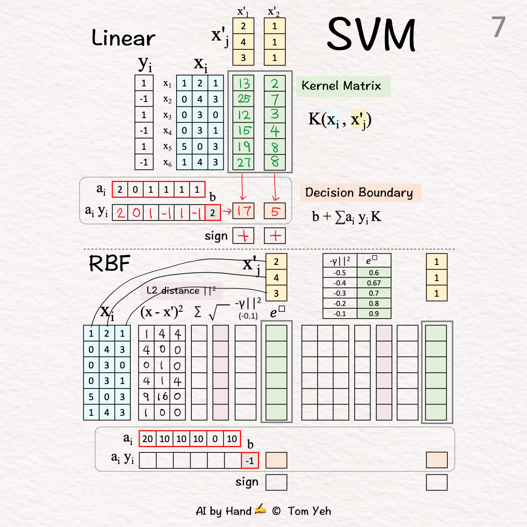
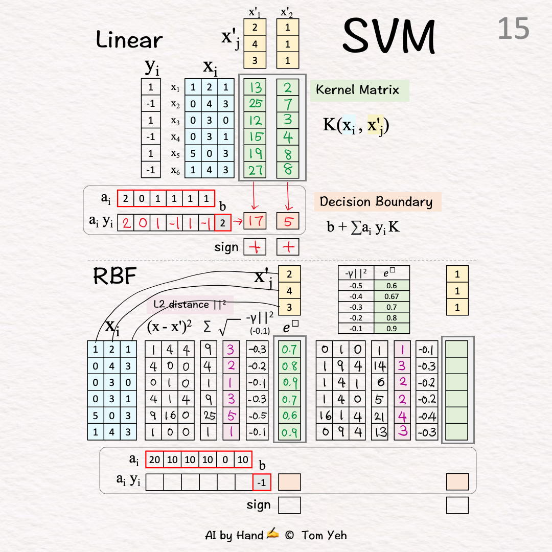
Support Vector Machines (SVMs) reigned supreme in machine learning before the ascendancy of the deep learning revolution.
This exercise compares Linear vs RBF SVMs---how they classify two test vectors, after SVMs are trained from six training vectors.

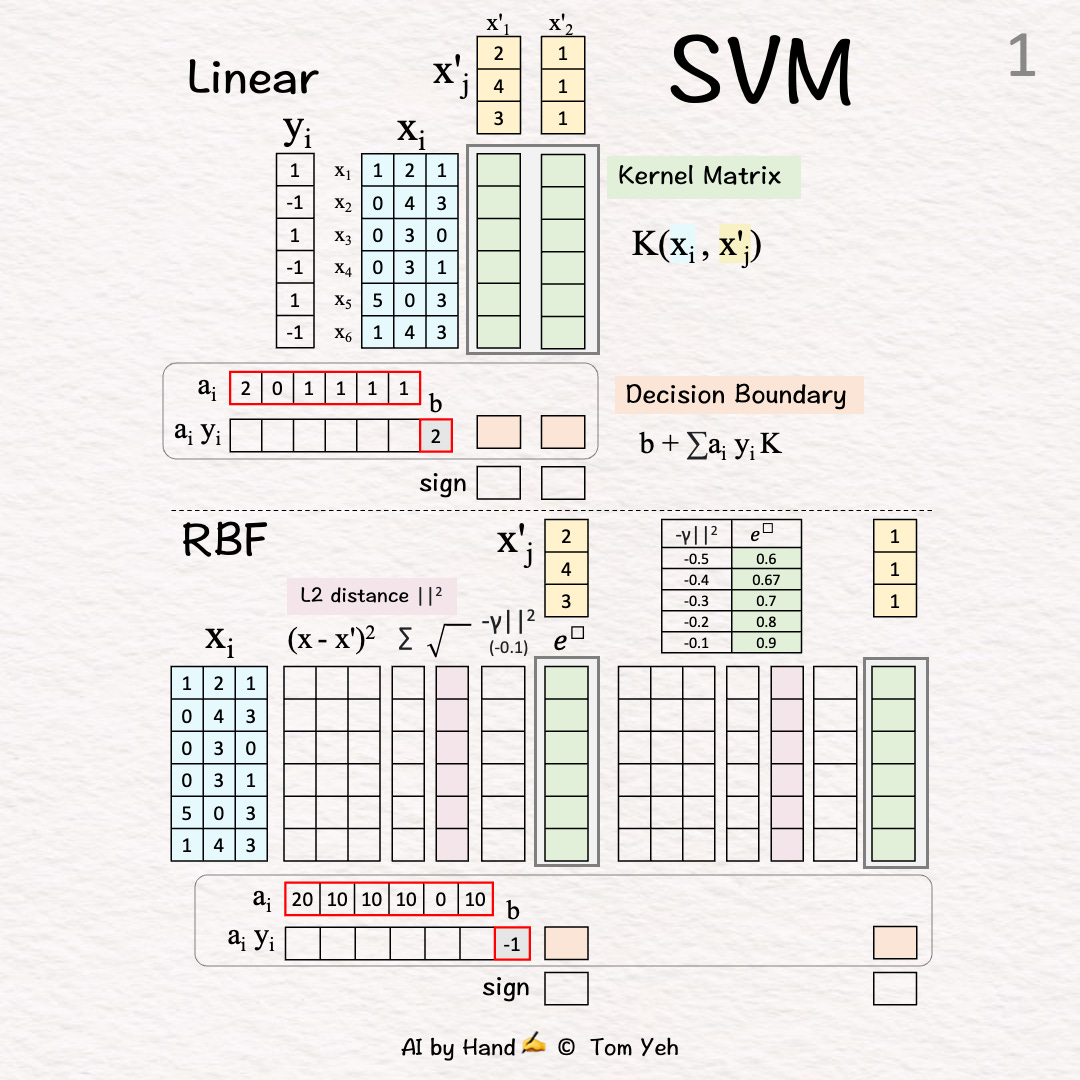
[1] Given
xi: Six training vectors (blue rows 🟦)
yi: Labels
Using xi and yi, we learned ai and b (red borders):
↳ai: coefficient for each training vector i.
• Non-zero: A Support Vector that defines the decision boundary
• Zero: Too far from the decision boundary, ignored
↳b: bias (how much the decision boundary should be shifted)
x’j: Two test vectors (yellow columns 🟨)
(To simplify hand calculation, training and test vectors are not normalized.)
🟩 Kernel Matrix (K) [2]-[3]
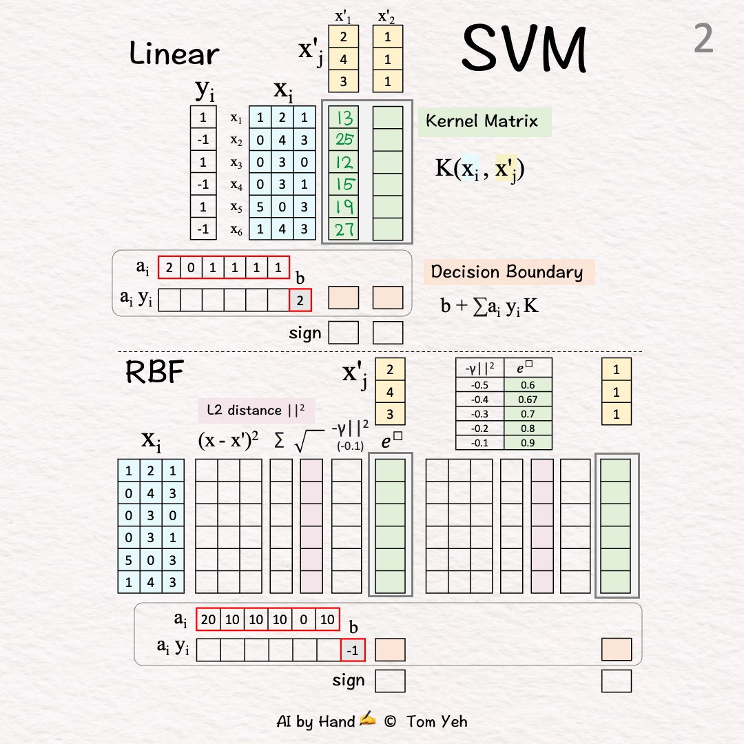
[2] Test Vector 1
↳ Take dot product between the test vector 🟨 and every training vector 🟦
↳ The dot product approximates the “cosine similarity” between two vectors
↳ Output: 1st column of K

[3] Test Vector 2
↳ Similar to [2]
↳ Output: 2nd column of K
🟧 Decision Boundary [4]-[6]
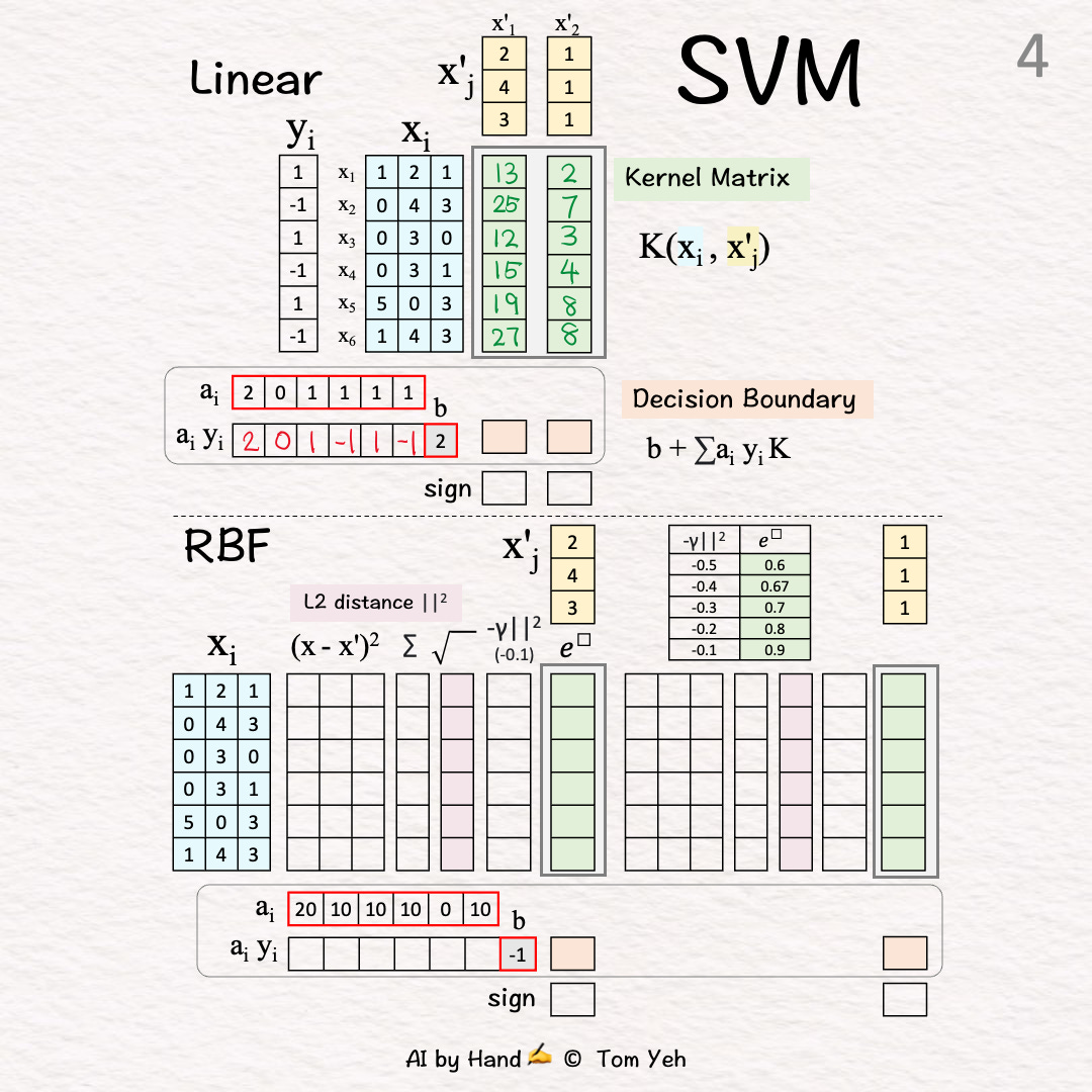
[4] Unsigned Coefficients → Signed Weights
↳ Multiply each coefficient with the corresponding label
↳ The 2nd training vector is NOT a support vector because its coefficient is 0.

[5] Weighted Combination
↳ Multiply weights and bias with K
↳ Output: “signed” distance to the decision boundary
X'1: (2)*13+0+(1)*12+(-1)*15+(1)*19+(-1)*27+(2) = 17
X'2: (2)*2+0+(1)*3+(-1)*4+(1)*8+(-1)*8+(2) = 5
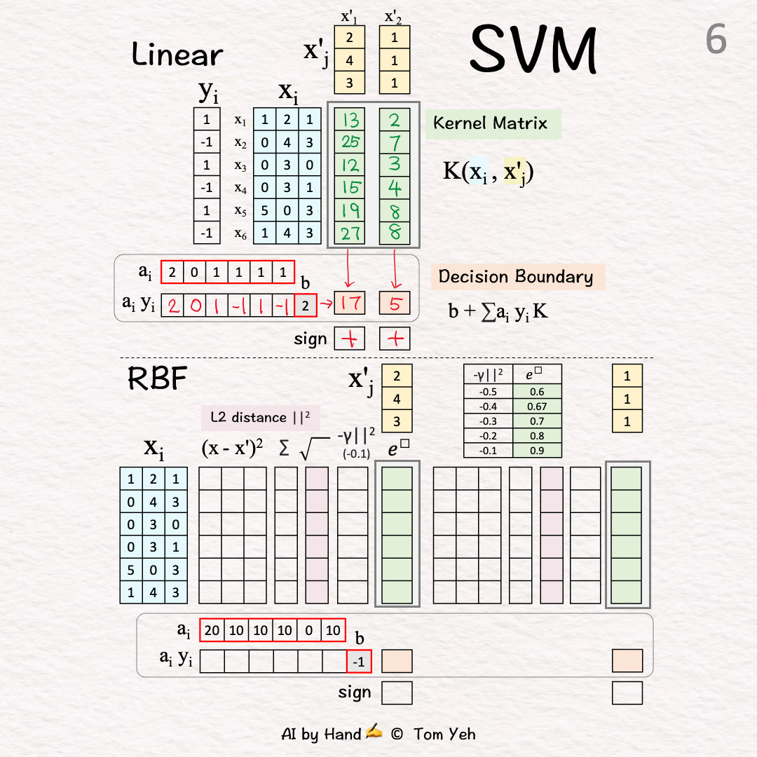
[6] Classify
↳ Take the sign
X'1: 1 > 0 →  Positive +
X'2: 5 > 0 →  Positive +
Given
ai: Learned coefficients
b: Learned bias
🟩 Kernel Matrix (K) [7]-[15]
Test Vector (X’1) 🟨
L2 Distance 🟪 [7]-[9]
[7] Squared Differencei=1: (1-2)^2=1, (2-4)^2=4, (1-3)^2=4
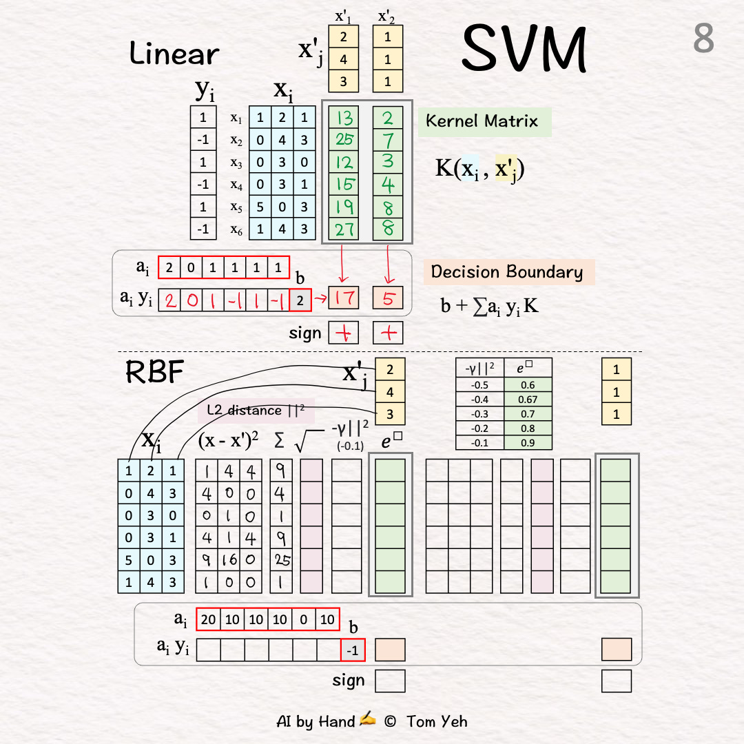
[8] Sum
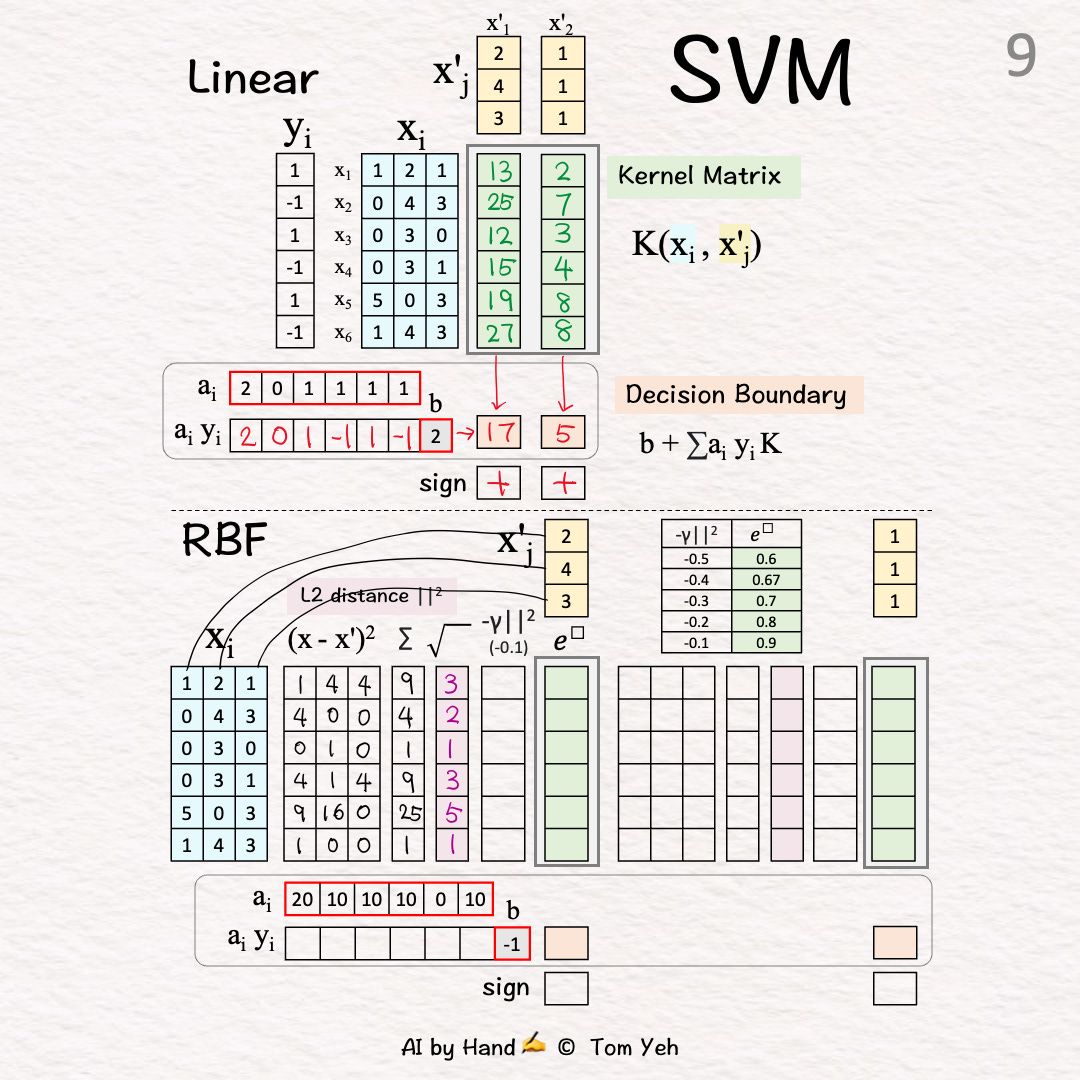
[9] Square Root
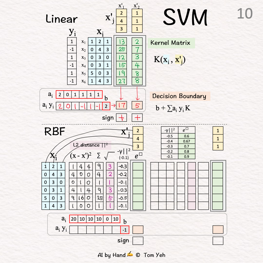
[10] Negative Scaling
↳ Multiply by -1: Note that L2 is a distance metric. The negation converts distance to similarity.
↳ Multiply by gamma γ: The purpose is to control how much influence each training example has. A small gamma means each training example pulls the decision boundary more lightly, resulting in smoother decision boundaries.
↳ The result is “negative scaled L2”
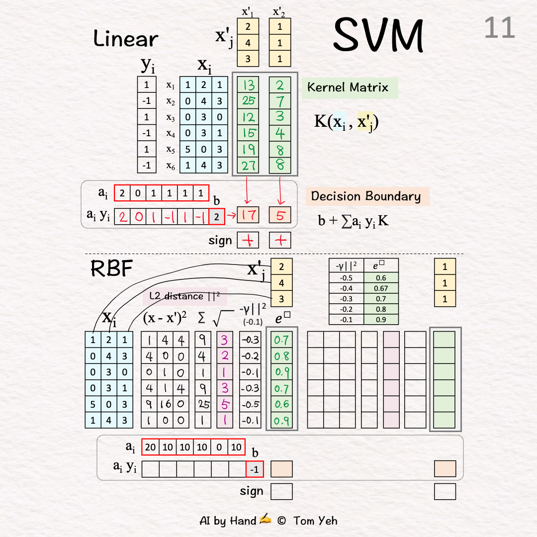
[11] Exponentiate
↳ Raise e to the power of the “negative scaled L2”
↳ Use the provided table to look up the value of e^
↳ Output: The 1st column of K
Test Vector 2 (X’2) 🟨
L2 Distance 🟪 [12]-[14]
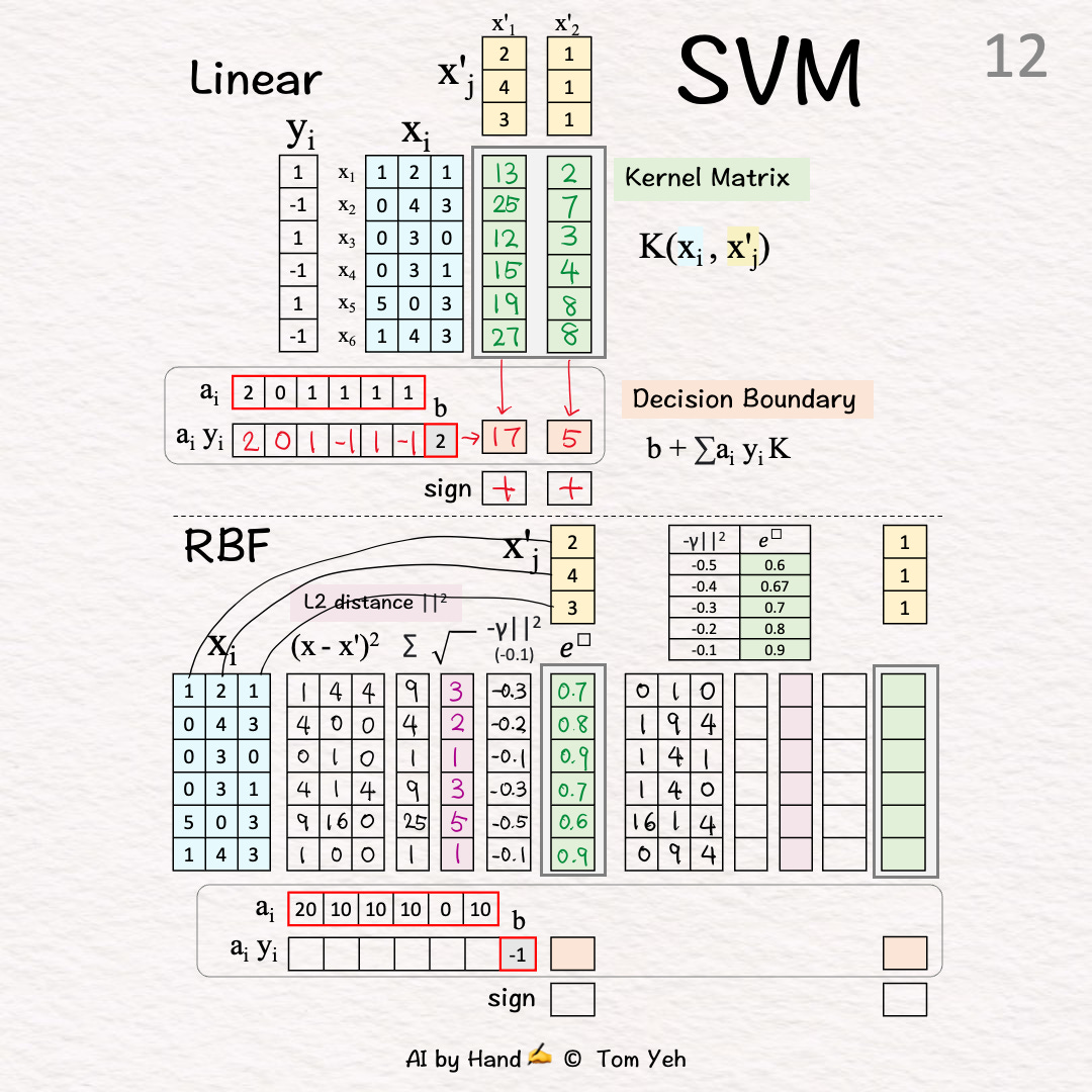
[12] Squared Difference
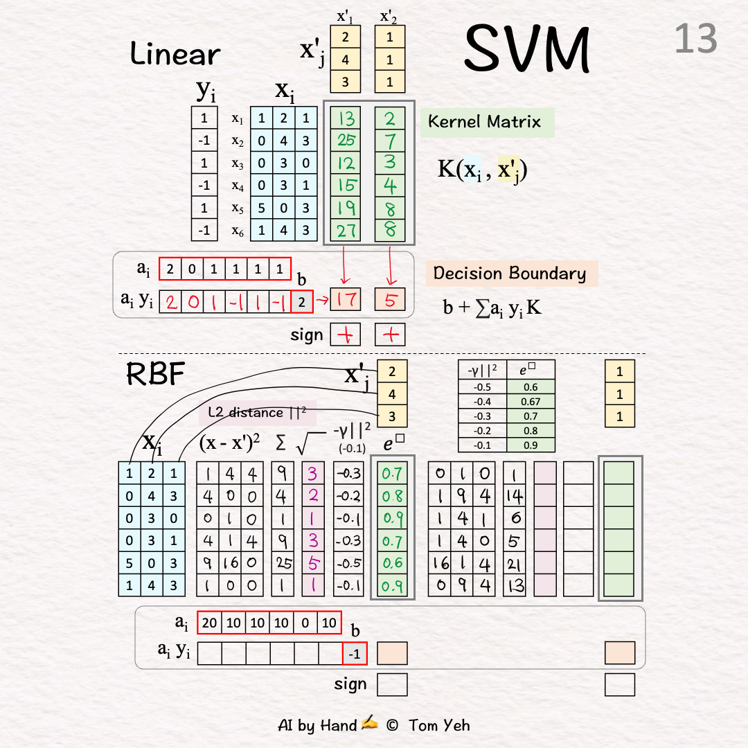
[13] Sum
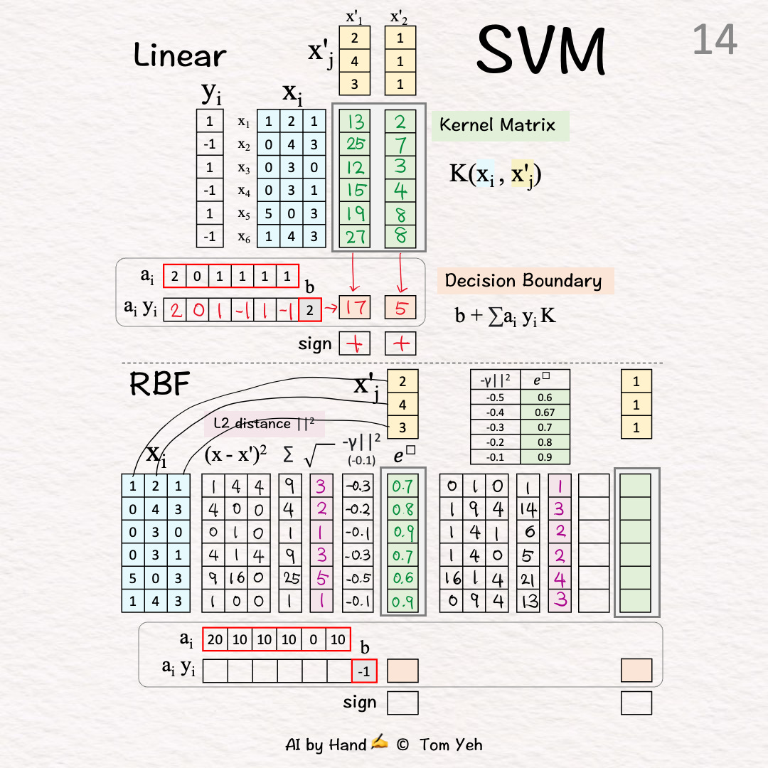
[15] Negative Scaling
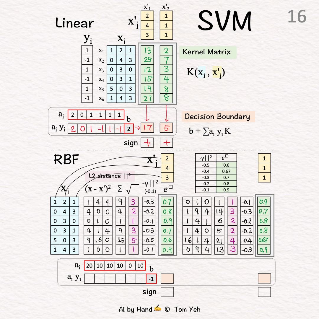
[16] Exponentiate
↳Output: The 2nd column of K
🟧 Decision Boundary [17]-[19]
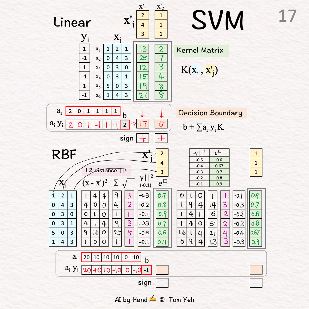
[17] Unsigned Coefficients → Signed Weights
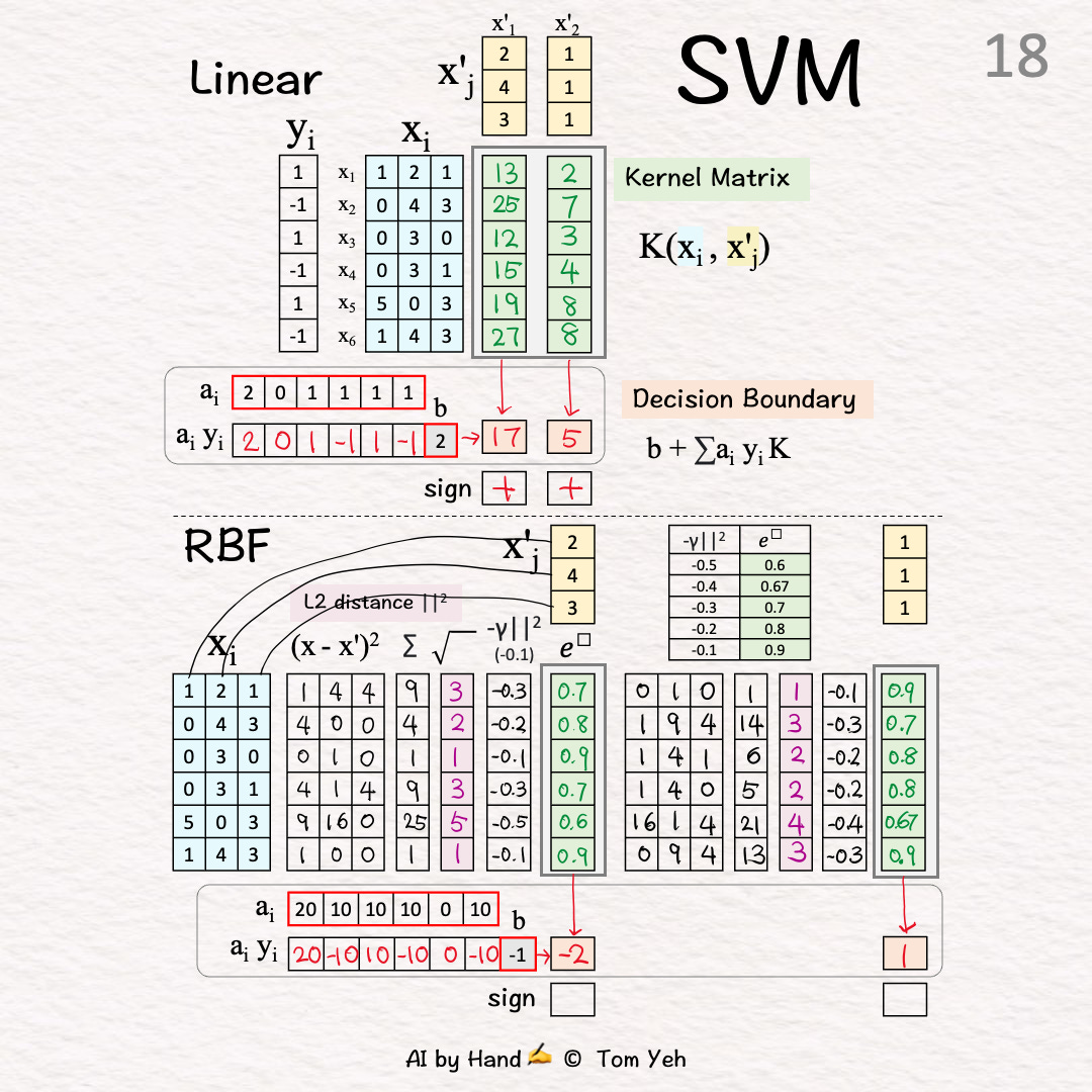
[18] Weighted CombinationX'1: (20)*0.7+(-10)*0.8+(10)*0.9+(-10)*0.7+0+(-10)*0.9+(-1) = -2
X'2: (20)*0.9+(-10)*0.7+(10)*0.8+(-10)*0.8+0+(-10)*0.9+(-1) = 1
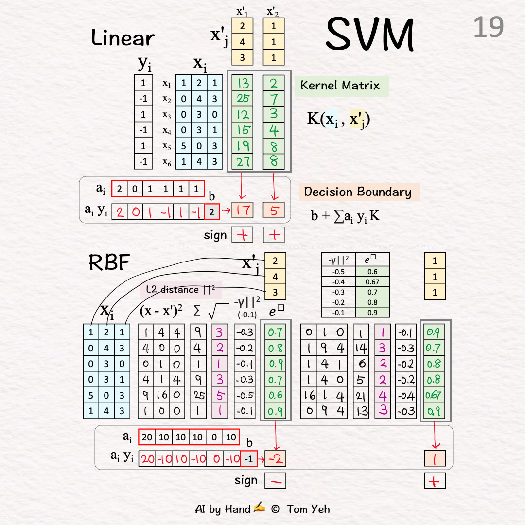
[19] ClassifyX'1: -2 < 0 → -
X'2: 1 > 0 → +