I’ve spoken several times about jittered Voronoi grids, such as here. These are infinite Voronoi diagrams where the sites come from randomly picking a point from each square in a square grid.


They’re simple and popular in procedural generation. But I’ve been a bit vague about computing them previously, and that’s because I was wrong.
You typically compute the infinite diagram lazily, one cell at a time. To compute a single cell, you take some neighbourhood of the cell, compute the finite Voronoi diagram using one of the many algorithms for that, and extract cell computed there. For a large enough neighborhood, this always gives the exact answer. But what is large enough.
I had previously assumed a 5×5 neighborhood was sufficient. So did proc gen master Inigo Quilez, and this SIGGRAPH paper.
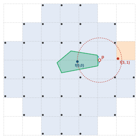
But it’s possible for any of the 36 cells shaded below to matter. This diagram shows why the (3, 1) site is important – the green polygon shows the Voronoi cell for the (0, 0) site computed with/without including the (3,1) site, it’s clearly different in each case. The red circle shows that, the closest site to p is the (3,1) site and the second closest site to p is the (0,0) site.
I wanted confidence this answer was finally correct, so I wrote a formal proof using Lean. I’ve been using Lean at work, and increasingly finding uses for it in my hobby work (here’s another one I did).
I don’t claim this is a new insight, it’s mentioned in A Vectorizable Random Lattice, Moukarzel–Herrmann 1992 and Performance of Random Lattice Algorithms, Lauritsen–Puhl–Tillemans 1993. But it seems very poorly known in the graphics community, and I wasn’t able to find a proof online.
Note: This is not the neighborhood you’d use for pixel shader approaches which just look for the nearest site, like Worley noise. Those only require evaluating the nearest 21 sites to the current pixel (or even fewer if you are smart about it).