Iran closed the Strait of Hormuz to commercial shipping on 28 February 2026. To measure what stopped moving, WherobotsDB read 719 Sentinel-2 scenes, 151 GB in total, straight from the public archive and fetched only about 1.5 GB covering three areas of interest. A near-infrared threshold found the hulls with no trained model, and a join against Overture Maps land polygons removed rocks and coastline. Traffic through the surveyed corridor fell 95% while loading and anchorage traffic held at 2025 levels, and the whole analysis cost about $63.
Sentinel-2 imagery is free and covers the planet every five days. Pointing the same job at another chokepoint takes two edited arguments.
What the satellites saw
We counted vessel hulls in Sentinel-2 imagery over three areas from January 2025 to August 2026 using a pixel-based reflectance method, while accounting for the sun’s angle over time:
| area | 2025 | 2026 | change |
|---|---|---|---|
| Hormuz transit corridor | 10.3 vessels | 0.5 | −95% |
| Fujairah anchorage, outside the strait | 63.5 | 70.0 | +10% |
| Kharg Island export terminal, inside the Gulf | 7.3 | 9.9 | +35% |
Those figures are per satellite pass, averaged over the passes clear enough to cover the whole area.
We used imagery because the usual source cannot be trusted here. Ship traffic is normally tracked through AIS, which is the transponder every large vessel carries. In this crisis those transponders are being switched off or falsified. Near Fujairah and Khor Fakkan, roughly 470 vessels broadcast garbled or impossible positions inside a single 24-hour window. Windward counted 146 of 167 vessels in the strait area running dark on 5 May, and IMF PortWatch warns that its own numbers understate traffic. The optical imagery provides a signal (the hull) that is always on.

How to count ships from space
Water absorbs almost all near-infrared light, so in Sentinel-2’s B08 band the sea is nearly black. Painted steel reflects it strongly. Over the Fujairah anchorage on August 7th, 2026 the water sat at 0.09 reflectance and the brightest pixel in the area read 0.87, so a vessel stands out by a wide margin. This means you don’t need a machine-learning model to identify a ship.
Wherobots queries the Sentinel-2 files directly in the public archive. The raster data source opens each scene in place and fetches only the necessary pixels.
The code below is an excerpt from the job script but the whole pipeline is available as a runnable notebook that opens in Wherobots Cloud, with every constant in one cell so you can point it at your own area of interest.
Show the code
AOI = ("POLYGON((56.42 25.10, 56.62 25.10, 56.62 25.30, "
       "56.42 25.30, 56.42 25.10))")
AOI_SQL = f"ST_SetSRID(ST_GeomFromWKT('{AOI}'), 4326)"

(sedona.read.format("raster")
    .option("tileWidth", "512").option("tileHeight", "512")
    .option("autoRescale", "true")      # off by default: without it you get raw DN
    .load(paths)
    .createOrReplaceTempView("tiles"))

# Background statistics on water only. The median centre ignores a bright
# minority of pixels. Pooling the per-tile standard deviations by their median
# discards a tile spoiled by cloud or land, but bright pixels inside a tile
# still inflate that tile's spread, so a crowded anchorage lifts the cutoff
# somewhat. That bias is conservative and falls on both years alike.
r = sedona.sql(f"""
    WITH s AS (
        SELECT zs.median AS med, zs.stddev AS sd
        FROM (SELECT RS_ZonalStatsAll(rast, {WATER_G}) AS zs FROM tiles)
        WHERE zs.count > 0
    )
    SELECT percentile_approx(med, 0.5) AS med, percentile_approx(sd, 0.5) AS sd
    FROM s
""").collect()[0]

threshold = r["med"] + max(SIGMA_K * r["sd"], 0.03)
2026-08-07 cov=100.0% cloud= 2.67% med=0.0915 sd=0.0097 thr=0.1687 \
brightpx= 5636 vessels= 84 >=200m= 39RS_ZonalStatsAll reports statistics for the pixels inside a shape. Using the median prevents a small number of bright pixels from raising the threshold; an average would be pulled upward by every ship in the frame. Adding a multiple of the spread gives a cutoff for that scene. The spread is pooled the same way, by taking the median of each tile’s standard deviation, which discards a tile spoiled by clouds. It is only a partial defense: ships inside a tile raise that tile’s spread, and with it the cutoff, so the count runs slightly conservative in a crowded anchorage. The sea is brighter in July than in January, so the cutoff has to move with it, which we account for in the analysis.
A short Python function applies that cutoff, and RS_Polygonize traces the outline of every bright patch.
Show the code
@sedona_vectorized_udf(return_type=RasterType())
def threshold_udf(rast: SedonaRaster) -> SedonaRaster:
    a = rast.as_numpy_masked()[0]
    out = np.zeros(a.shape, dtype=np.float64)
    with np.errstate(invalid="ignore"):
        out[np.isfinite(a) & (a >= threshold)] = 1.0
    return rast.with_bands(out[np.newaxis])


# with_bands() needs real pixels; the reader returns out-db references.
(sedona.sql("SELECT RS_AsInDB(rast) AS rast FROM tiles")
    .withColumn("mask", threshold_udf("rast"))
    .createOrReplaceTempView("masked"))

# RS_Polygonize returns every connected region in ONE array, so running it on a
# whole scene OOMs an executor -- per tile it is cheap and parallel.
sedona.sql(f"""
    SELECT t.p.geom AS g
    FROM masked LATERAL VIEW explode(RS_Polygonize(mask, 1)) t AS p
    WHERE t.p.value = 1.0
      AND ST_Area(t.p.geom) BETWEEN 2000 AND 200000
""").createOrReplaceTempView("raw_blobs")


# A vessel lying on a tile seam is polygonized twice, once either side of the
# cut. Union everything, then split it back apart: the halves become one
# polygon, while vessels that never touched stay separate. The area floor above
# runs before this merge, which has a cost the last section spells out.
sedona.sql("""
    WITH dissolved AS (
        SELECT explode(ST_Dump(ST_Union_Aggr(ST_MakeValid(g)))) AS g
        FROM raw_blobs
    ),
    sized AS (
        SELECT g, ST_Area(g) AS area_m2,
               2 * ST_MinimumBoundingRadius(g).radius AS length_m,
               ST_MinimumWidth(g) AS width_m
        FROM dissolved
        WHERE ST_Area(g) BETWEEN 2000 AND 200000
    )
    SELECT g AS geometry, area_m2, length_m, width_m
    FROM sized
    WHERE width_m >= 20
      AND length_m / width_m BETWEEN 2 AND 15
""").createOrReplaceTempView("candidates")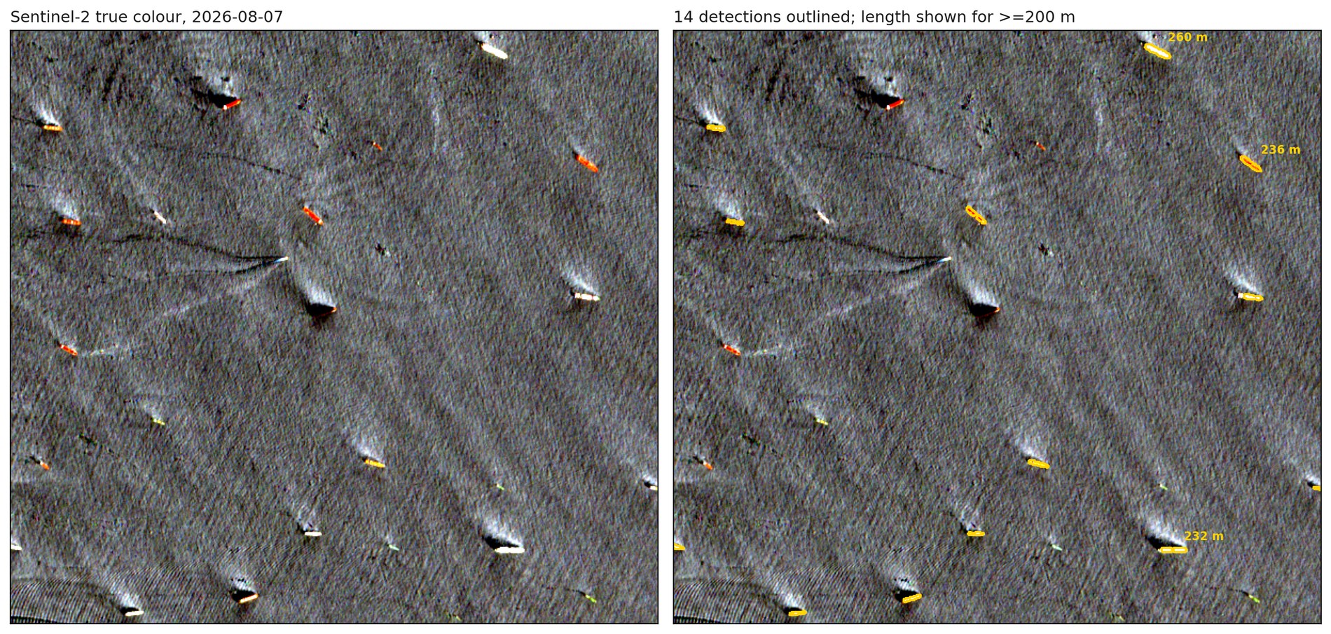
Ruling out rocks, land and glint
Rocky islets also reflect near-infrared light. The Quoin Islands sit directly in the shipping lane, and in an early run three of our first four detections turned out to be those rocks.
Wherobots holds imagery and map data in one engine, so checking detections against an independent source takes one query. Overture Maps publishes global land polygons. They already sit in the Wherobots open data catalog, and one join drops any detection that touches land.
Show the code
sedona.sql(f"""
    SELECT ST_Buffer(ST_Transform(geometry, 'EPSG:4326', 'EPSG:{epsg}'), 60) AS g
    FROM wherobots_open_data.overture_maps_foundation.base_land
    WHERE ST_Intersects(geometry, {AOI_SQL})
""").createOrReplaceTempView("land")

detections = sedona.sql("""
    SELECT d.geometry, d.area_m2, d.length_m
    FROM candidates d
    LEFT ANTI JOIN land l ON ST_Intersects(d.geometry, l.g)
""")
Two further checks run alongside it. Sun glint can brighten patches of open water, so we keep only detections shaped like ships, which filters out glint using the near-infrared band alone. A hull is typically four to eight times longer than it is wide and a glint patch is round, so the filter accepts anything between 2:1 and 15:1 and at least 20 m across. Those bounds are deliberately loose, wide enough that an unusual hull still passes while a round blob cannot. And a satellite pass sometimes covers only part of an area, so any date where less than 95% of the area was photographed is dropped. Counting a partly covered area would look like a decline in traffic that never happened. In practice nothing landed in between: every date behind the figures came in at 100% coverage, and the rest were dropped outright.
A study fusing Sentinel-1 radar with AIS measured a 97% decline across the two weeks either side of the closure. We measured 95% from optical imagery over a longer window, with no AIS involved.
Oversized shapes and the size bound
About one detection in forty measures longer than 400 m, a length no ship afloat reaches. The longest spans 1,310 m. These shapes cluster by date: at Fujairah, 15 of the 21 fall on a single date, and in the corridor, 13 of 24 fall on two, which fits cloud or sun glint on those passes. At Kharg, a shape about 1,120 m long recurs at the same spot on five dates, which points to a fixed terminal structure missing from the land polygons. An upper bound alongside the existing area floor removes all of them:
WHERE length_m BETWEEN 50 AND 400The correction tightens the result. The corridor returned nine detections on 18 March 2026, one of the two clustered dates, and five of those exceed 400 m. Four hulls survive the bound, so the corridor reads emptier after the closure.
Every vessel we found
The job writes its detections as GeoParquet and then as PMTiles, a single file a browser can read directly from cloud storage without a tile server. Each month becomes its own layer, so a before-and-after comparison means publishing the two months that matter.
Show the code
from wherobots import vtiles

feats = sedona.sql("""
    SELECT geometry, aoi, obs_date, length_m, area_m2,
           date_format(to_date(obs_date), 'yyyy-MM') AS layer
    FROM det
""")

vtiles.generate_pmtiles(feats, f"{base}/hormuz_monthly.pmtiles")
The three maps below show one area each, with the 2025 month in blue and the 2026 month in red. Each caption gives the month’s total and a per-pass rate, which divides that total by the number of usable passes.
The corridor. May 2025 in blue against May 2026 in red. 46 detections across four clear passes in 2025, then two across one pass: about 11 vessels a pass, down to two. Open fullscreen.
The anchorage outside. April 2025 in blue against April 2026 in red. 200 detections over three passes, then 122 over two, which is roughly 67 a pass and then 61. April appears here because no May 2026 pass covered the anchorage. Open fullscreen.
The loading terminal inside the Gulf, May 2025 in blue against May 2026 in red. Loading held: 22 detections over two passes in 2025 and 29 over three in 2026, or 11 a pass then about 10. Open fullscreen.
All three areas at once, with every month switched on: 3,117 detections in 20 layers, one per month from January 2025 to August 2026. Kharg sits to the north-west, the strait and Fujairah to the south-east. Step through the months in the sidebar to see the corridor empty while the anchorage and the terminal keep their traffic. Open fullscreen.
Compute cost and data read
719 Sentinel-2 scenes cross these three areas over 20 months, which is 151 GB of imagery. The analysis read about 1.5 GB of that, because RS_Clip fetches only the parts of each file that overlap the three areas. The scenes stay in the public archive throughout.
The 20-month run took 26.8 minutes on a MEDIUM runtime, roughly 25 Spatial Units at $1.50 each in us-west-2, or about $37. Widening the same job to the whole Gulf of Oman and lower Persian Gulf, 368,875 km² at full coverage, added $23 and seven minutes of wall clock. Calibration and tiling took it to about $63. Wherobots Cloud reports the exact figure for every run in Workload History.
The coordinates and date range are parameters, so pointing the job at another chokepoint is an edit to two arguments. The notebook has them in its configuration cell, alongside the size and shape limits. Sentinel-2 passes overhead every five days, and a scheduled run keeps the count current independent of AIS broadcasts.
The surveyed corridor is 25 km wide within a strait roughly 40 km across, so the 95% decline describes that corridor. Whether some vessels shifted to routes outside it cannot be settled from these three areas. A second limit sits in the detector. The 2,000 m² area floor runs before the seam merge, so a small hull lying on a tile boundary can split into two pieces that each fall under the floor and go uncounted. A hull touches a seam on roughly 2% of passes, the loss bites only near the size floor, and it applies to every date equally, so the year on year comparisons survive it. The downloadable notebook applies the area floor after the merge instead.