Here are the main takeaways from SmolLM’s recent playbook if someone is planning to train a new LLM (<10B) model from scratch in 2025, I’ve tried to keep it as concise as possible, and might have omitted things covered in the blog.
Architecture:
If you want a dense model, you can’t really go wrong with **Qwen3 or Llama3.1/2**. If you want to venture into MoEs, there is GPT OSS-20B, Qwen3-Next and Kimi moonlight. There’s also Kimi k2 but that’s more of a 32B scale.
Despite a lot of changes, most of the world shares the same foundation, which is like a decoder-only model. There are some variations with the attention mechanism, interleaving normalization and moe-level details, but the core remains the same.
To make ablating with the architecture more simpler, start off with a simple dense model similar to Qwen3 and Llama3, and then slowly build up to other kinds of models like MoEs and hybrid models.
How to Save on Parameter Size, while preserving most parts of the Arch
Embedding (Input + Output): Consider switching from tied to untied embeddings (doubles embedding parameters) (this works better for smaller models than larger counterparts as embeddings take lesser space in large models, 3% in 70B vs 13% in 8B). The untied one does similar (on unnoticeable gaps) performances as tied on smaller models in the ablations.
Attention mechanism: Going from MHA to GQA or MQA reduces parameter size heavily.
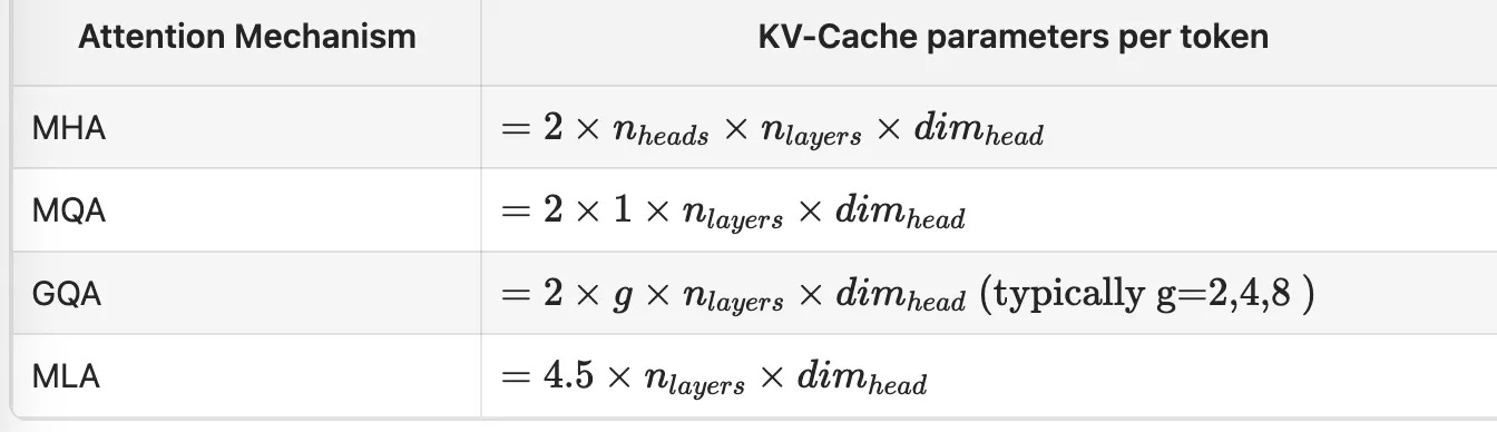
Based on the ablations (data mix being fixed) done in the blog, group query attention is a solid alternative to multi-headed attention. It preserves performance while being more efficient.
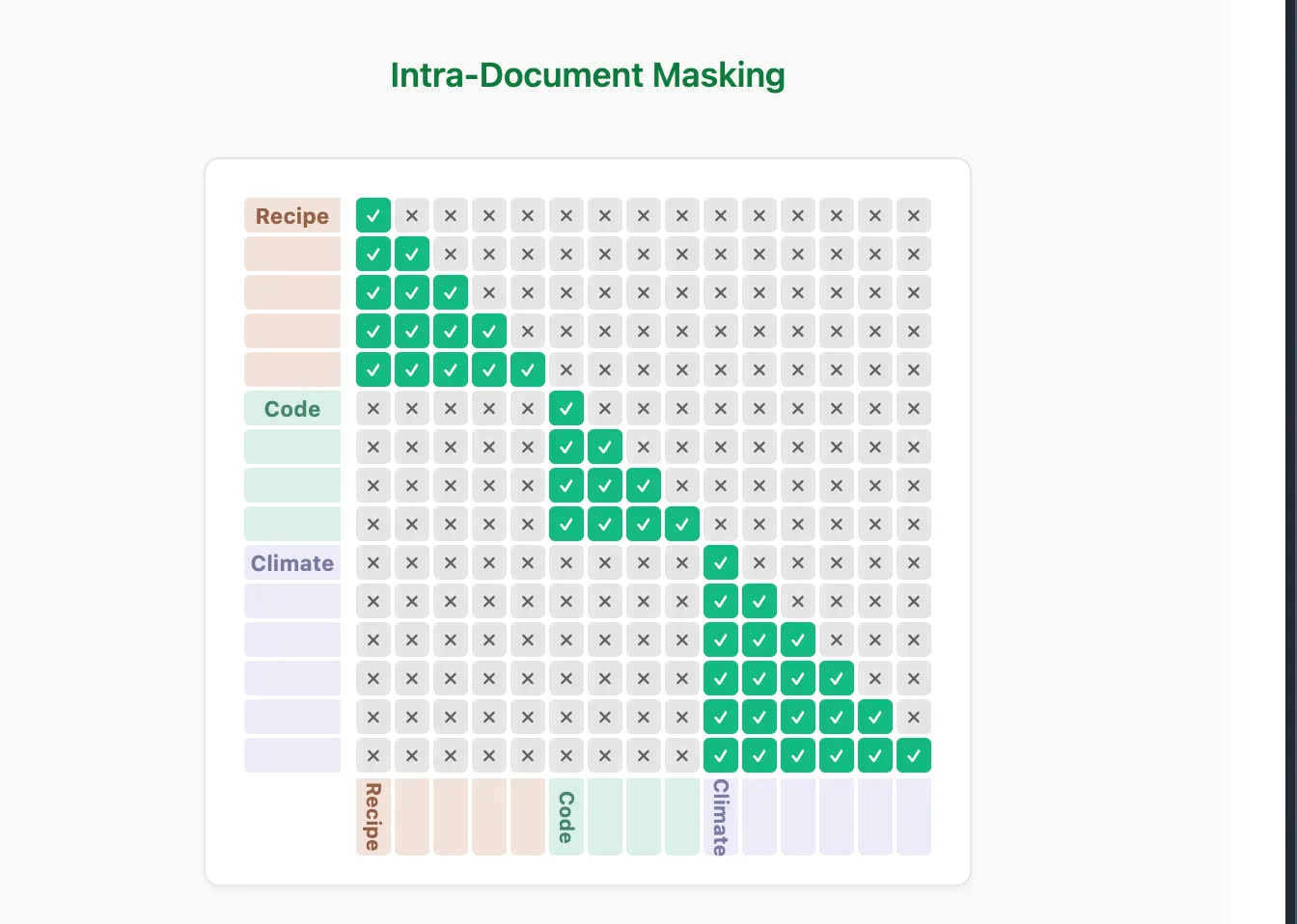
SideNote: Document Masking
Document masking essentially allows you to train for documents which have variable lengths with fixed training sequences. You can use packing i,e shuffle and concatenate documents with end-of-sequence tokens and split the result into fixed-length chunks, this allows you to have separate documents but all in one sequence. You can enable intra-document masking, which basically allows you to attend to only previous tokens with respect to the document while sharing the same attention matrix, so tokens from document B don;’t attend to tokens from document A, when both are concatenated. The mask applied to cross-doc attention weights.
Use of positional embeddings.
****I think there’s a lot of variations in positional embeddings, since gpt2 came out. We started off with absolute positional embeddings, moved towards relative positional embeddings, saw the use of alibi (which modifies attention based on token distance) until we converged (or relatively converged) on RoPE, that provided a way to extend LLMs to longer context lengths. Most major models today use RoPE (with or without adjusting base freq): Llama, Qwen, Gemma, and many others. RoPE has proven robust across different model sizes and architectures (dense, MoE, Hybrid).
There are other variants such as RoPE, which is like no positional embeddings, which also have shown some improvements like YaRN, however it remains to be tested more widely despite showing better performance in long-context scenarios. YaRN allows us to apply scaling factors to different frequency components, dynamic attention scaling and temperature adjustment. There are also other positional embeddings such as NoPE, removing positional embeddings completely, some works show that this can yield comparable results, but might lag behind in short-form content/generation lengths. Alternating NoPE with RoPE can give better gains on memory without compromising performance (3:1 ratio for example).
Use of attention scope/ Attention Modifications
To increase context length and/or reduce memory consumption, we have several variants of attention. There exists sliding window attention which sorts of attends to only the most recent tokens. There’s dual chunk attention which extends like chunk retention maintaining cross chunk information flow. Recently we’ve also seen the use of attention sinks where the model assigns high tensions to initial token to the sequence even when the tokens aren’t important., this can help in maintaining attn distrubutions in long context scenarios.
Tokenization.
The size of your vocabulary depends on the size of the model. For smaller models (1-3B) and English-only models, 50,000-60k tokens suffices, and multilingual requires double of that.
For English-only models, around 50k tokens usually suffices, but multilingual models often need 100k+ to efficiently handle diverse writing systems and languages. Modern state-of-the-art models like Llama3 have adopted vocabularies in the 128k+ range to improve token efficiency across diverse languages.
People still use BPE mostly. But there are some existing works which have adopted sentence piece and word piece as well. There is also some renewed interest in tokenizer-free algorithms. To evaluate tokenization, you can use the metrics like fertility, which just takes the average number of tokens to encode a word. The lower the better, so there’s less fragmentation when words are tokenized (per language).
When to use existing tokenizers: If your target use case matches the language or domain coverage of the best tokenizers above (Llama, Qwen, Gemma), then they are solid choices that were battle-tested.
When to train our own: If you’re training for low-resource languages or have a very different data mixture, we’ll likely need to train our own tokenizer to ensure good coverage. In which case it’s important that we train the tokenizer on a dataset close to what we believe the final training mixture will look like.
Optimiser and training hyperparameters
Learning Rates
It’s a good idea to stick to AdamW, while there are other variants that might seem enticing at the time (Muon). This is primarily because how well-tuned/tested AdamW is across model families, especially for long runs.
The learning rate is one of the most important hyperparameters we’ll have to set. At each training step, it controls how much we adjust our model weights based on the computed gradients. Choosing a learning rate too low and our training gets painfully slow and we can get trapped in a bad local minima. The loss curves will look flat, and we’ll burn through our compute budget without making meaningful progress. On the other hand if we set the learning rate too high we cause the optimizer to take massive steps that overshoot optimal solutions and never converge or, the unimaginable happens, the loss diverges and the loss shoots to the moon.
People have been using cosine annealing for a while, where I start at a peak learning rate and then smoothly decrease following a cosine curve. There are new variants used by papers like DeepSeek where you don’t have to start decaying immediately:
Warm up stable decay
Multi-step
You maintain a constant high learning rate for most of training, and either sharply decay in the final phase (typically the last 10-20% of tokens) for WSD, or do discrete drops (steps) to decrease the learning rate, for example after 80% of training and then after 90% as it was done in DeepSeek LLM’s Multi-Step schedule.
In ablations, however, the warm-up, stable decay matches cosine with small models, and you could go with either of them.
Batch Size
Batch size is another important factor that plays a role in speeding/slowing up training as we vary our learning rates. A bigger batch size allows a better estimation of the gradient but is more computationally expensive as well. if we scal e the abtchsize by k, we need to prortionally reduce the learning rate by sqrt(k) as well, if we want to keep the variance constant, and variance is proportional to the learning rate times inverse of batch size.
Beyond a certain point, larger batches start to hurt data efficiency: the model needs more total tokens to reach the same loss. The breakpoint where this happens is known as the critical batch size, and you need to stay below this.
Increasing the batch size while staying below critical: after increasing the batch size and retuning the learning rate, you reach the same loss with the same number of tokens as the smaller batch size run, no data is wasted.
Increasing the batch size while staying above critical: larger batches start to sacrifice data efficiency; reaching the same loss now requires more total tokens (and thus more money), even if wall-clock time drops because more chips are busy
Scaling Laws for HyperParams
The optimal parameters for our training go beyond our learning rate and batch size. There are some emperically derived scaling laws for how model perf evolves with more training data. We can expend compute in either parameters or data, and given a total compute budget C, the relationship between the three looks like:
C≈6×N×D
N is the number of model parameters (e.g., 1B = 1e9), D is the number of training tokens. This is often measured in FLOPs (floating-point operations). The constant 6 comes from empirical estimates of how many floating-point operations are required to train a Transformer, roughly 6 FLOPs per parameter per token (calculation includes estimation for forward/backward pass, estimation etc).
Note: Models are trained longer, and for more tokens often labelled as ‘overtrained’ even for their relatively small sizes <3B params. training duration is often dictated by the amount of compute available. You can choose to train beyond the scaling law described above at your own discretion and needs.
Pre-training Data Mixes
A mix of high-quality datasets that provide early signal across a wide range of tasks. For English (FineWeb-Edu), math (FineMath), and code (Stack-Edu-Python) (Total 45B in tokens). A good rule of thumb could be 30-40B tokens for small models like 1-3B range. For data ablations you should fix the architecture first and then vary the data-mix. What should be the proportions of the data mix? A mix of FineWeb-Edu and DCLM, can comprise 5.1T of tokens, and ablations show that a 50-50 or 40-60 mix can provide the best balance across benchmarks.
Mixing multilingual data:
Adding multilingual data to english mixes without degrading the performance can be a challenge, and to try this a good rule of thumb is to keep multilingual mix to be lesser than 20% of the primary data.
Through ablations on the 3B model, we found that 12% multilingual content (*600B tokens) in the web mix struck the right balance, improving multilingual performance without degrading English benchmarks
How does the data mix evolve with the training curriculum
We start off from the stage 1 mixture we outlined above, making it 40% of the new mix, and then leaving 60% of the new mix to be the experimental candidate we want to measure.
You should add data like math and code are added in later training stages, like midtraining and post-training.
Training FAQs
How to deal with loss spikes?
Recoverable spikes: These can recover either fast (immediately after the spike) or slow (requiring several more training steps to return to the pre-spike trajectory). You can usually continue training through these. If recovery is very slow, you can try rewinding to a previous checkpoint to skip problematic batches.
Non-recoverable spikes: The model either diverges or plateaus at worse performance than before the spike. These require more significant intervention than simply rewinding to a previous checkpoint.
Common culprits, assuming a conservative architecture and optimizer, include:
High learning rates: These cause instability early in training and can be fixed by reducing the learning rate.
Bad data: Usually the main cause of recoverable spikes, though recovery may be slow. This can happen deep into training when the model encounters low-quality data.
Data-parameter state interactions: PaLM (Chowdhery et al., 2022) observed that spikes often result from specific combinations of data batches and model parameter states, rather than “bad data” alone.
Poor initialisation: Recent work by OLMo2 (OLMo et al., 2025) showed that switching from scaled initialisation to a simple normal distribution (mean=0, std=0.02) improved stability.
Precision issues: While no one trains with FP16 anymore, BLOOM found it highly unstable compared to BF16.
Some other fixes if spikes still persist after diagnosing the issue:
Skip problematic batches : Rewind to before the spike and skip the problematic batches. This is the most common fix for spikes.
Tighten gradient clipping : Reduce the gradient norm threshold temporarily
Apply architectural fixes such as QKnorm (layer normalization to both the query and key vectors before computing attention). Normalisation before the attention computation helps.
Midtraining
Modern LLM pretraining can be seen through multiple stages than just a single pass over the training data-mix. Each stage imparts different purposes, from general purpose knowhow, to reasoning, and long-context generalization.
If you need to make the model as generally capable you can tailor the later two stages in pre-training accordingly. The data mixture doesn’t have to stay fixed throughout training. Multi-stage training allows us to strategically shift dataset proportions as training progresses. Often Stage 2 mixture will contain high quality math and code data to impart reasoning, this would be same as pretraining but more on the domain relevant datasets.
An example of the 3 stages is outlined below:
Stage 1: Base training (8T tokens, 4k context) Using pretraining mixture: web data (FineWeb-Edu, DCLM, FineWeb2, FineWeb2-HQ), code from The Stack v2 and StarCoder2, and math from FineMath3+ and InfiWebMath3+. All training happens at 4k context length.
Stage 2: High-quality injection (2T tokens, 4k context) Using higher-quality filtered datasets: Stack-Edu for code, FineMath4+ and InfiWebMath4+ for math, and MegaMath for advanced mathematical reasoning (we add the Qwen Q&A data, synthetic rewrites, and text-code interleaved blocks).
Stage 3: LR decay with reasoning & Q&A data (1.1T tokens, 4k context) During the learning rate decay phase, further upsampling high-quality code and math datasets while introducing instruction and reasoning data like OpenMathReasoning, OpenCodeReasoning and OpenMathInstruct.
Note: Long Context Training
For enabling long context training, if youre using something like RoPE, you can adjust base frequencies as you increase the context length of the documents you train on.
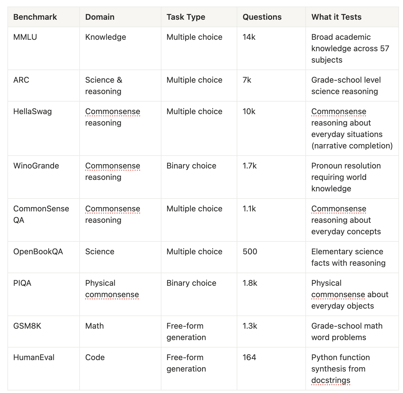
Evals (for pretraining and final ckpts)
Post-training
A lot of what goes into the modern capabilities of models like instruction following or reasoning that get people excited appear more naturally once we post-train them.
You can use a mix of following recipes as a part of post-training (not necessarily use all)
Supervised fine-tuning (SFT) to instil core capabilities.
Preference optimisation (PO) to directly learn from human or AI preferences.
Reinforcement learning (RL) to refine reliability and reasoning beyond supervised data.
Data curation to strike the right balance between diversity and quality.
Evaluation to track progress and catch regressions early.
Start off with SFT, Cold Starting the RL runs with SFT is becoming more and more common place with RL runs, and we see that with Qwen, Kimi, Olmo and the likes. It is also much more cost effective and easy to curate the supervised data pairs for question and answers needed to do SFT on a model.
Some example datasets that you can include in your mix:
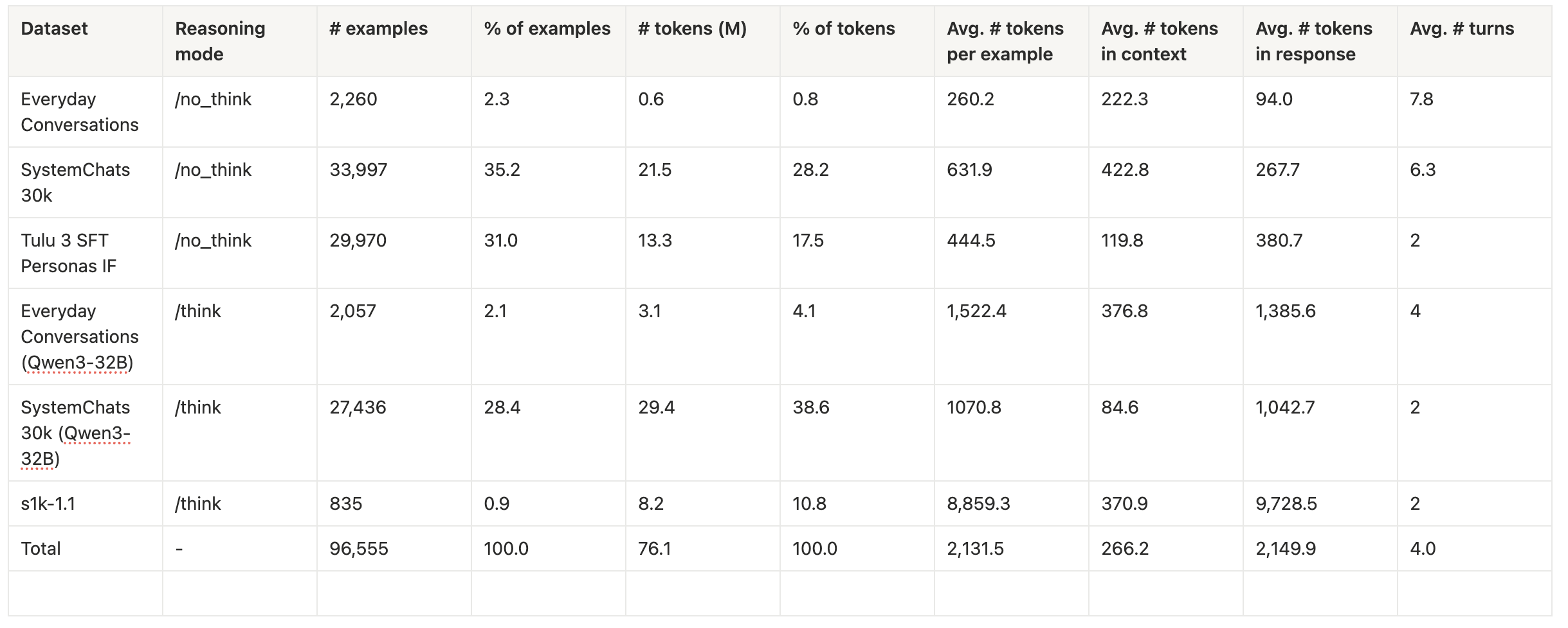
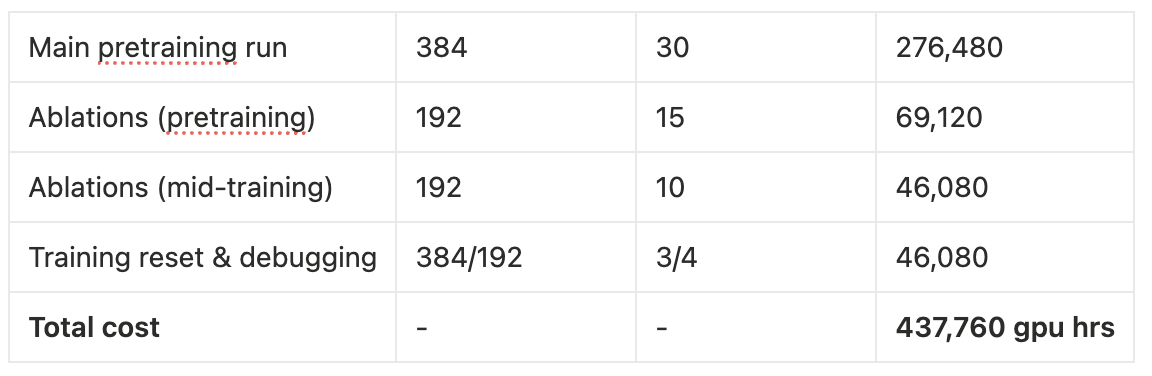
Cost (for a 3B model)
One of the most interesting (and gpu poor moments) was looking at what sort of cost was for the training run, ablations and the debugging. This was almost 440,000 GPU Hours, which would translate to a 1M-2M USD (if you calibrate like one GPU per hr on a H100 as $2.2-4 USD per hr). Considering the money people raise pre-seed for ai-startups, it might be actually viable to train at least a few custom models (if really needed be)