For a CPU architect who is used to innovations that are increasingly incremental and “in the details”, the range of solutions in ML accelerators is impressive: radically different approaches coexist here at the same time. They answer the same fundamental problems in different ways, and each challenges the dominance of GPUs in its own way.
While ML software is evolving rapidly, each chip is basically becomes a fixed in silicon hypothesis about future workloads. But what will future ML workloads look like, and whose bet will work better?
ML software does not evolve in a vacuum: available hardware “highlights” some directions as practical and scalable, while making others expensive - the hardware lottery effect. As a result, hardware specialization can not only satisfy demand, but also direct the evolution of algorithms and models, and maybe to theoretically suboptimal state. This brings us back to the need for HW/SW co-design.
One of the central needs for HW/SW co-design is coming from the fact that the classic CPU model with a cache-coherent shared address space increasingly runs into the cost of data movement. When a byte becomes more expensive than a FLOP, then locality, data movement, and the question of who manages on-chip memory become critical: hardware (caches) or software/compiler (scratchpads).
Time ago in the CPU world VLIW approach challenged OOO by moving scheduling from dynamic hardware into the compiler and was not very successful. And now again we face the dilemma of “how much complexity to keep in hardware, and how much in software”. Today a similar logic appears in dataflow / explicit-memory approaches, where efficiency is achieved not by prediction and caches, but by planning of compute and data movement. Is there now a greater chance of success with this approach, given that ML-software is much more specialized and adaptable?
In this article, I want to build for myself a map of the key architectural directions and trade-offs in ML hardware — a framework that helps compare different designs, understand what bets they make, and what drives them — and then maybe reflect a little bit on ML hardware evolution. As an “index”, I will start from the properties of ML workloads that make them different from general-purpose computing, and look at typical architectural choices that follow from these properties. I intentionally stay with relatively proven, production-oriented approaches, and do not touch more exotic ideas like neuromorphic chips, photonics, or compute-in-memory (maybe come back to that in the future).
In ML, much of the work can be expressed as a relatively small set of tensor primitives — matmuls, convolutions, reductions, normalizations, and a variety of elementwise and layout/format transforms. This has a straightforward implication: we can build compute that is not fully universal, but extremely efficient for these primitives with specialized units.
Оptimizing the matmul in isolation is rarely enough. End-to-end performance is often limited by what happens between large matrix operations: normalization and activation chains, softmax, reductions, reshapes/transposes, quantize/dequantize, and other glue that tends to have low compute-per-byte. If these pieces are slow or if they force intermediate tensors to be written out to external memory, the system underperforms and burns bandwidth and energy on traffic rather than doing useful work.
That brings us to the need for fusion.
Consider a MatMul followed by a Quantization step: Without fusion, the full result of the matrix multiplication is written to memory, only to be read back (sometimes even by a different processor, like the CPU) to perform quantization and write it yet again. In a fused implementation, as soon as a tile of the result is computed and still resides in the accelerator’s local registers/SRAM, we apply quantization immediately. This eliminates the massive overhead of reading and writing intermediate structures to external memory.
Specialized units mainly make compute cheaper (faster matmul, reductions, special functions, etc.). Fusion of nearby compute stages mainly makes data movement cheaper. You can do fusion even on fairly general hardware, but without fusion you often have to write intermediate tensors to HBM/DRAM and read them back right away — and then even specialized compute units end up waiting for bytes.
The practical goal is simple: keep intermediates on-chip (registers/SRAM), run common operator chains as one fused step, and write only the final result to external memory.
That is why accelerators usually pair tensor/MAC engines with “support” blocks: vector/SIMD for elementwise work, fast reductions (sum/max/mean), SFU/SFPU for exp/rsqrt/tanh, and layout/format helpers (transpose/permute, pack/unpack, cast/quantize). These blocks are not decoration — they are what makes real fused graphs fast, not only standalone GEMM benchmarks.
Specialized units are everywhere, what differs is their mix and balance.
For illustration, AWS NeuronCore-V3 has four compute blocks:
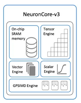
Tensor Engine — optimized for tensor computations such as GEMM, CONV, and Transpose.
Vector Engine — optimized for vector computations, where each element of the output tensor depends on multiple elements of the input tensor. Examples include AXPY operations (Z = aX + Y), Layer Normalization, and Pooling operations.
Scalar Engine — optimized for scalar computations, where each element of the output tensor depends on one element of the input tensor.
GPSIMD engines — each GPSIMD engine consists of eight fully programmable 512-bit-wide vector processors. They can execute general-purpose C code and access the embedded on-chip SRAM, which allows implementing custom operators and executing them directly on the NeuronCores.
As been mentioned, we need fusing to reduce the number of times we move and store intermediate tensors — that’s one of the keys optimization related to Memory Wall problem: in many ML workloads, bytes are more expensive than FLOPs.
In ML, the bottleneck is often not compute, but data movement.
A clear example is LLM inference, where a single workload switches between two phases with opposite bottlenecks. During prefill, the model processes the entire input prompt in parallel — large matrix operations with high arithmetic intensity, comfortably compute-bound. During decode, the model generates tokens one at a time: we read the full weights (tens to hundreds of gigabytes) plus the growing KV cache just to produce a single token. This is brutally memory-bound — tensor cores sit idle, waiting for bandwidth.
The asymmetry creates a design tension. A GPU is well-utilized during prefill but overpowered for decode: most of its FLOPS capacity goes unused while it waits on HBM. SRAM-centric architectures can potentially win on decode latency when weights fit on-chip — but this requires sharding across many chips, and then chip-to-chip interconnect may become the new bottleneck. The memory wall doesn’t disappear; it moves to a different level of the hierarchy. Software responds with batching — larger batches mean better weight reuse during decode, pushing it closer to compute-bound. But batching adds latency: each request waits for the batch. Real-time chat wants minimal batching; offline processing wants maximum. Techniques like continuous batching and chunked prefill try to balance this, but the fundamental mismatch : optimizing for one phase often means compromising the other.
Besides that, real graphs also contain many operators with low compute-per-byte — layernorm/softmax, reductions, and layout/format transforms (transpose/permute/cast/quantize). These steps generate extra traffic and can become bandwidth-bound even when the main matmuls look compute-heavy on paper.
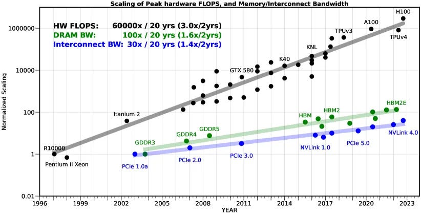
This problem will likely intensify. Over the past 20 years, peak server hardware FLOPS has been scaling at 3.0×/2yrs, outpacing the growth of DRAM and interconnect bandwidth, which have only scaled at 1.6 and 1.4 times every 2 years, respectively. This disparity has made memory, rather than compute, the primary bottleneck in AI applications, particularly in serving.
Capacity is also a bottleneck: in training, memory is consumed by gradients, optimizer state, and activations; in inference, on top of the weights you also have the KV cache, which grows with context length and the number of sessions, and you want to keep the working set close to compute. The capacity wall almost always turns into a bandwidth wall — because spilling/offloading/sharding adds extra data movement and synchronization.
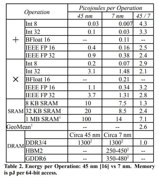
However, the Memory Wall in ML is not only about bandwidth and capacity, but also about energy cost. In fact, moving data can consume much more energy than the compute itself
At a high level, there are three ways to organize memory and data movement for ML (and they can be combined):
Buy bandwidth close to compute (HBM-heavy packages)
Use HBM and advanced packaging (2.5D/3D) to put high-bandwidth memory very close to the accelerator. This gives great bandwidth and better energy per bit, and it is easier to keep a “shared memory” programming model. But the cost is also high: price/complexity, power density, thermals/DVFS (meanwhile, cooling eats up from 7% to over 30% of total energy consumption in data centers), and limited in-package capacity. This looks like a short-term solution, since the demand for bandwidth keeps growing.
Examples: GPUs, AWS Inferentia/Trainium, Google TPU
Keep the working set on-chip and stream data (SRAM-first / dataflow-like)
Instead of relying on a big shared memory, use local SRAM/scratchpads and move data explicitly between compute blocks (often in a planned, push-based producer→consumer way instead of cache predictive magic). This can reduce external memory traffic and latency, but it usually needs a stronger compiler/runtime and a stricter HW/SW contract.
Examples: Tenstorrent, Graphcore IPU, SambaNova. Groq is related, but more rigid: the compiler fixes a static schedule, closer to a VLIW-like approach and, in some sense, to Jacquard loom.
Hierarchy and distribution
HBM + DDR (+ NVMe), streaming/prefetch, compression, sharding/placing the KV cache across accelerators. But this creates pressure on the interconnect and makes planning more complex.
The Memory Wall is one of the main problems: in ML, bytes become expensive, so both software and hardware constantly look for many other ways to reduce traffic and the working set — via fusion, pruning/sparsity, mixed precision and quantization. Next, we will look at these aspects as well.
ML workloads offer a lot of parallelism — inside operators (matrix tiles, vectors, wraps) and at the system level (batches, many requests, model/pipeline parallelism). We can use this parallelism to scale compute throughput, but there is a catch: more parallel compute needs more data movement. If we cannot deliver enough bytes per second (from memory and across the interconnect), extra compute simply waits for bandwidth.
So parallelism is not only “how many MACs we can run at once”. It is a system question: how we feed those MACs, how far the bytes have to travel, and what it costs in latency, energy, packaging complexity, and cooling.
There are two practical tasks here:
Choose an execution model (parallelism + memory semantics)
This choice starts with the execution model: SIMT (GPU-like), MIMD/task-based, or dataflow/spatial. It defines the basic work unit (warp / task / tile stream) and how much scheduling is static vs dynamic. But it also defines the memory contract. SIMT systems typically assume a shared address space with caches and latency hiding, while dataflow/spatial systems rely on explicit local buffers/scratchpads and planned data movement.
Then comes another axis: granularity and irregularity. Do we optimize for large regular tiles (throughput), or for many small quanta (warp/tile/task) to handle ragged batches and conditional compute?
Scale the system so that this model does not run into memory / packaging / interconnect limits
Scaled compute has to be fed by a memory hierarchy (SRAM ↔ HBM ↔ DDR/NVMe) and by links between dies and between accelerators. And once we try to bring more bandwidth “close to compute” (HBM, wider interfaces, 2.5D/3D), packaging and thermals become part of the performance story.
For this map, I split “execution / parallelism models” into two layers. The first table covers operator-level (in-core / datapath) styles — how a single kernel (like GEMM or elementwise) is executed. The second table covers system-level execution styles — how work is scheduled across many cores/tiles and how data is moved between them.
A useful shortcut is to read each model along three axes:
Memory semantics: cache-heavy shared memory vs explicit local SRAM/scratchpads
Scheduling: mostly static (compiler plan) vs more dynamic (runtime balancing)
Granularity: large regular tiles vs many small quanta (warps/tasks) to handle irregularity
A) In-core and datapath styles (operator-level parallelism)
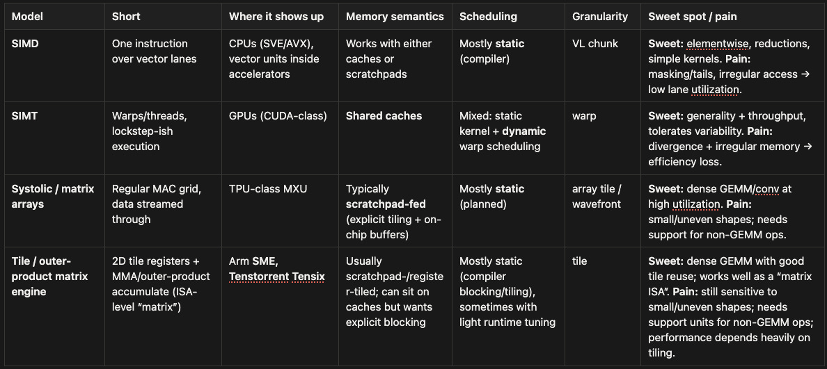
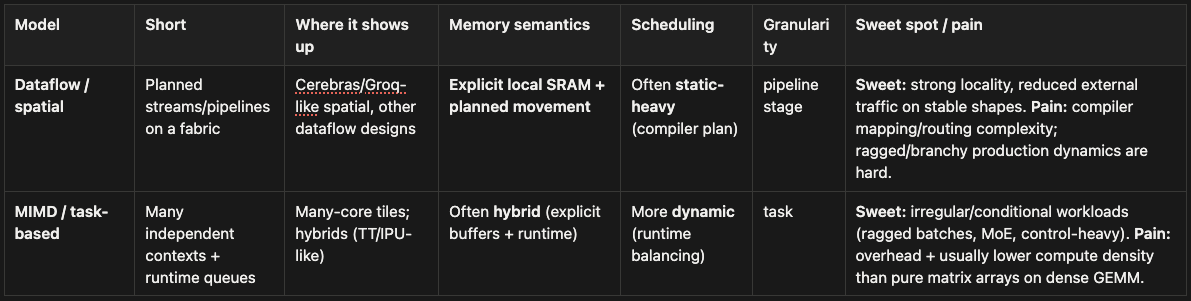
B) System execution styles (graph-level execution + data movement)
Real accelerators are usually hybrids: tensor engines + SIMD/SIMT-style support units + some mix of dataflow and task scheduling.
For example, Tenstorrent-style design can combine a dataflow-style plan (explicit data movement and planned exchanges) with MIMD execution on programmable cores which include a tile-based matrix engine plus SIMD/vector support.
As soon as we really try to utilize parallelism, we discover that we need to scale not only compute, but also what feeds it: interconnect and memory — and after memory, packaging as well.
To overcome the Memory Wall (see the previous section) and feed scaled compute, we have to choose (or combine) several memory types:
Off-package DRAM (DDR/LPDDR) — cheap and high-capacity, but with lower bandwidth and higher latency. Matmuls are “fed” only if locality / tiling / prefetch are done well.
HBM — very high bandwidth — HBM3 is “terabytes per second” (≈3 TB/s per accelerator), while DDR5 is “hundreds of gigabytes per second” (≈0.1–0.6 TB/s per socket) — and better pJ/bit thanks to a wide interface. With HBM it is easier to stay with a “big shared memory” model. The price: more expensive / more complex packaging, higher power density near compute (→ DVFS, energy for cooling), and limited in-package capacity.
On-chip SRAM (cache/scratchpad) — minimal energy per bit and high speed, but expensive in area, so capacity is limited and requires careful planning.
Packaging is basically a memory trade-off: “electrically closer” vs “thermally lighter”.
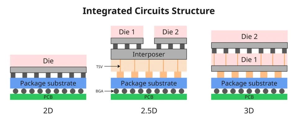
2D package: chips sit on a plane, DRAM is off-package → easier thermals, but lower bandwidth.
2.5D (interposer): chips still sit side by side on a plane, but communicate through a high-density interposer. Convenient HBM integration and wide interfaces → better BW/latency, but higher cost/complexity and higher power density.
3D stacking: chips are stacked on top of each other — even closer and wider, but the thermal path is worse (upper layers make heat removal harder), so thermal risks grow and sustained performance becomes more constrained.
As parallelism grows, the interconnect becomes part of the computation: it defines the cost of synchronization, activation/parameter exchange, and the efficiency of collective communication operations.
Interconnect scales hierarchically:
On-die Network-on-Chip (NoC): the internal network that connects compute blocks, L2/SRAM, memory controllers, etc.
In-package die-to-die (chiplets): the “network inside the package” can become part of the critical path; at the same time, it scales the “atom” of the accelerator.
Off-package links (PCIe, NVLink, InfiniBand, Ethernet): connect multiple accelerators into a node/cluster.
Two typical scaling paths:
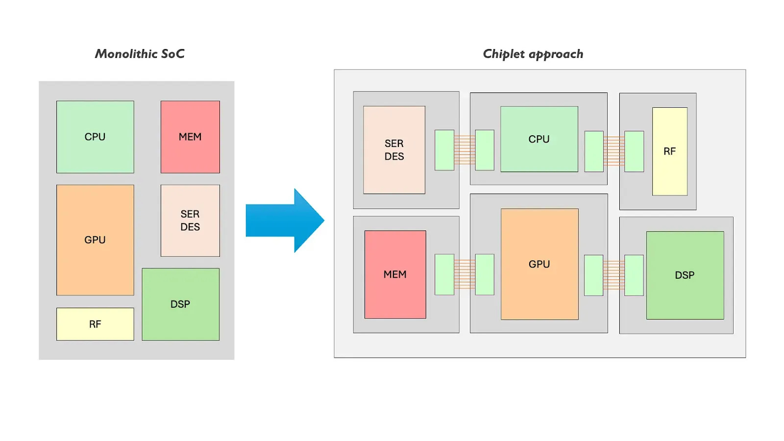
Monolithic: fewer “seams” → simpler latency/determinism/synchronization, but we hit the economics and physics of a large die, and then — the network at scale. Two-level communication: NoC → external network.
The most radical example is Cerebras: a chip that uses (almost) the whole wafer.

Chiplets / multi-die: better yield/cost and more flexible composition; we can compose more elements, even with different technologies. Communication becomes three-level: NoC → die-to-die fabric → off-package links, but the die-to-die interconnect can become a bottleneck for sustained performance (BW/latency limits and NUMA effects).

In general-purpose computing, calculations are usually exact and predictable. In ML, a different trade-off is often acceptable: models can tolerate a controlled loss of precision if it does not significantly affect quality, and in return it can give a multiplicative gain in throughput, energy, and (especially) memory bandwidth / capacity (this helps both compute and the Memory Wall).
That is why ML hardware is built around:
BF16/FP16 as the baseline modes,
FP8/INT8 as more aggressive modes for speedup and saving memory/traffic,
INT4 mostly as a storage format (weights, sometimes KV cache), usually with compute done in a wider format,
wide accumulation: we multiply in a “narrow” format, but accumulate partial sums in FP32/INT32 to keep numerical stability.
This creates a whole ecosystem: data formats, converters, and compiler policies that decide where it is safe to go narrower, and where it is not.
CPUs historically target a very broad class of workloads and “unexpected” runtime behavior: unpredictable branches, addressing patterns, and cache behavior. That is why the architecture invests heavily into prediction (branch predictors, caches, prefetching) and dynamic scheduling.
In ML the situation is often different: the computation topology and the operator set are usually known in advance, and inside operators we often have a regular loop structure. This opens an opportunity to replace part of prediction with longer-range planning: the compiler can choose tiling and scheduling ahead of time, plan buffer reuse (memory planning) and organize data movement so that compute blocks spend less time waiting for memory.
This is exactly where specialized accelerators get a window of opportunity against GPUs: instead of the universal “threads + shared memory + caches” model, they can rely on explicit memory / scratchpads and a more static datapath — up to dataflow ideas and even a “VLIW-like” approach, where a significant part of control moves from hardware into the compiler. That is why such designs appear: Groq, Tenstorrent and others.
However, production workloads bring back dynamics and irregularity (different request lengths, RAG, mixed batches, branching, MoE). So a single “perfect static plan” is not enough: we need an architecture that combines compilation with runtime adaptation and cheap scheduling of small work units.
So, an “ideal static plan” is useful, but not always sufficient and we need an architecture that can both compile well and adapt.
In many models and operators, sparsity appears and it is something we can potentially optimize.
In ML, sparsity can appear in different forms: value sparsity (e.g., pruned weights), activation sparsity (zeros produced by nonlinearities such as ReLU), and pattern/structural sparsity (e.g., attention masks that forbid certain query–key pairs).
Sparsity can be static or dynamic. Static sparsity is known in advance (for example, sparse weights after pruning) and is easier to optimize. Dynamic sparsity depends on the input (activations, MoE, etc.) and requires cheap detection and planning — otherwise the benefit is eaten by overhead.
In practice, sparsity is useful only if we can achieve both (a) less traffic and/or less compute, and (b) not drown in overhead.
Not “random zeros anywhere”, but zeros in blocks or in a pattern. Then it is easier to use matrix units, overhead is lower, and load balancing is simpler. This is a typical HW/SW co-design: hardware supports a few convenient patterns, and pruning/training/compiler adapt to them.

Example: NVIDIA 2:4 structured sparsity support (2 of 4 elements are zeroes).
If a block of data is zero, or its contribution is known to be zero, we can avoid reading/transferring/writing it further. If it is not zero, but there are many zeros, compression/quantization may work. The win here can be even larger than “skipped MACs”, because in ML moving bytes is often the expensive part.
If we can skip computations for zero/forbidden regions (weights, activations, attention masks) — we skip them. But this works only if skipping happens in large chunks or very cheaply; otherwise “accounting for zeros” starts to cost more than the compute itself.
Sparsity almost always brings a “side tax”: we need to store masks/indices, reads become irregular, and the workload becomes imbalanced (some places have many non-zeros, others almost none). If we do not compensate for this, part of the cores sit idle and the whole benefit disappears.
Sparsity, like scheduling, often reduces to granularity: at what block size we exploit it. Larger blocks are simpler and cheaper to skip (and the “tax” is smaller), but the sparsity is used less precisely. Smaller blocks give more potential savings, but the risk of drowning in overhead is higher.
In some systems sparsity is handled locally and in a specialized way (separate blocks/paths for sparse operations, like in TPU), while in others (Tenstorrent) there is a bet on broad support for sparsity and conditional execution as one of the core principles of the architecture and runtime.
Conditional compute means that not the whole graph is executed every time: the set of blocks used for a particular token/request is selected on the fly. This adds irregularity: different amount of work for different tokens, more small fragments and synchronizations.
Examples:
MoE — a token is routed to a subset of experts → load imbalance and (sometimes) extra communication.
Early-exit / block-level pruning — some layers are skipped → data-dependent branching.
Speculative decoding — parallel generation + accept/rollback → uneven control flow.
Agent / tool-use — more logic and external steps, often with I/O.
This is where a GPU can be less efficient: divergence increases, memory accesses become more irregular, and batching works worse. That is why some accelerators look for wins not in “even wider SIMD/SIMT”, but in cheap scheduling of small tasks and a more MIMD / task-based execution model, often combined with explicit memory / scratchpads (a clear example is Tenstorrent).
In the CPU world, the ISA and the basic contract live for decades. In ML, everything is different: key patterns and favorite operators have already changed several times (for example, ConvNets → Transformers, dense models → MoE, precision formats), and they will keep changing.
The evolution continues even within established architectures. Attention mechanisms that seemed canonical a year ago are being replaced by variants that trade compute for memory or avoid the KV cache entirely. Hardware optimized for today’s attention patterns may find itself mismatched tomorrow — another reason why the software stack matters as much as the silicon.
The whole dilemma comes down to what workload assumptions we bake into hardware. A DSA (domain-specific accelerator) can deliver a big jump in perf/W and cost per token — but only while the workload stays close to what it was optimized for. With rapid model/workload evolution, such designs risk losing their advantage in “steps”: graph shapes change, the share of non-GEMM work shifts, and we get more conditional compute and more irregular production dynamics.
The general-purpose approach (the GPU pole) pays a constant tax for universality (control/scheduling/memory system), but it is usually more robust: it stays “good enough” as patterns change, even if it is never optimal.
Then economics enters the picture: sometimes CAPEX (buy and integrate) matters more, sometimes OPEX (energy/cooling/utilization) and the final cost per token dominates. So the “best” design depends on the horizon: how fast it must pay back before the next wave of rapid evolution.
Finally, a long-term durable advantage is more often created not by the datapath itself, but by the quality of the stack around it: how quickly the compiler/runtime can adopt new operators and new modes (precision, sparsity, scheduling), and how convenient it is to run all of this in production. In ML, the compiler and runtime are not an accessory — they are part of the architecture.
SIMT (GPU-style), systolic/matrix engine (TPU-style), dataflow/spatial (Tenstorrent, Cerebras…), MIMD/task-based hybrid (Tenstorrent) — a choice between density/simplicity vs flexibility/adaptation.
Which ops we accelerate in hardware and how much we can fuse: vector/SIMD, reductions, exp/rsqrt, layout/format transforms, softmax/norm, etc.
Cache-heavy (hardware-managed) vs explicit memory / scratchpads (compiler/runtime-managed) vs hybrid approaches (some levels are caches, some are managed buffers/DMAs).
HBM-heavy package (buy bandwidth via packaging) vs SRAM-first + streaming/push dataflow vs system-level working set (HBM+DDR(+NVMe), KV placement, compression/quantization).
How much execution and transfers are fixed by the compiler in advance, and how much freedom is left to hardware/runtime.
Large tiles (throughput) vs small quanta (warp/tile/task) to keep utilization high on uneven sizes and with conditional behavior / sparsity.
On-die NoC, in-package die-to-die (chiplets), off-package links (PCIe/NVLink/IB/Ethernet). Scaling granularity: monolithic (fewer seams, simpler latency/determinism, but limited by big-die physics) vs chiplets (better yield/flexibility, but die-to-die fabric becomes a potential bottleneck).
How aggressively we use advanced packaging for BW/latency, accepting limits on sustained performance and thermals.
BF16/FP16 as the baseline, FP8/INT8 as aggressive modes, INT4 mostly for storage; plus wide accumulation and compiler policy about where it is safe to go narrower.
Structured patterns vs more general block/tile-level approaches; “don’t move” (compression/skip transfers); “don’t compute” (skip MACs); and again granularity, so overhead does not eat the win.
MoE/early-exit/speculative/tool-use → architecture/runtime optimized for irregularity: cheap fine-grained scheduling, smaller penalty for branching/imbalance, good support for ragged batches vs overhead on all that.
How domain-specific the hardware assumptions are vs how much the bet is on the stack (compiler/runtime/autotuning/tooling) to stay robust under rapid evolution and adopt new ops/modes without new silicon.
If we step away from details, here is the high-level picture: an ML accelerator is not only a datapath, it is a contract between silicon and the software about who is responsible for what. Some designs hard-code the rules in hardware, others leave more freedom to the compiler and/or runtime — and pay for that with corresponding overheads. The constraints are almost always the same: bytes are more expensive than FLOPs, and an “ideal” scheme breaks under production irregularity if it cannot keep utilization high. That is why different architectures look so different: they distribute the pain differently across memory, control, and planning.
Today the market leader is NVIDIA: GPU as a universal compute engine (SIMT + tensor blocks) with a strong stack, where performance is often “bought” with memory and packaging — HBM, complex packages, heavy thermals and power delivery.
Next to it, there is a second pole: hyperscaler accelerators (Google TPU, AWS Inferentia/Trainium, and others) that accept similar trade-offs, but tighten hardware and software around their typical scenarios to win efficiency at scale.
Pressure around HBM (bandwidth/capacity/energy) and the general “cost of a byte” created a third pole — SRAM-centric and dataflow/spatial approaches (Groq, Tenstorrent, SambaNova, Graphcore IPU, etc.), where the goal is to reduce traffic more aggressively and keep data closer to compute. This is not only research exotics: recent deals and partnerships around Groq and Cerebras suggest that non-GPU inference is becoming a strategic topic even for the big players.
A plausible scenario: the GPU share will decrease first in inference (memory/communication, cost-per-token, irregularity and conditionality of production workloads), while in training GPUs will likely keep their position longer thanks to universality, a mature stack (CUDA), and proven scaling. At the same time, the shift in inference will probably start with relatively universal “hybrids”, and more “pure” dataflow architectures may win later — if patterns and tools stabilize.
Dataflow/SRAM-centric designs still have pain points: working-set capacity (weights + KV cache, growing linearly with context length and number of sessions and the quadratic cost of self-attention with context length) often push the system back into external memory and network; plus production irregularity makes static planning expensive and increases the cost of compiler/runtime mistakes. But software also impacts on what the “best architecture” looks like: if we move away from transformer attention with large KV toward new attention schemes or alternative model families, the bottleneck profile will shift — and the window for dataflow may widen.
And my most subjective point: out of all ideas, the most elegant one (to my engineering taste) looks like the Tenstorrent bet (and no, I have no relation to them): dataflow/spatial with explicit data movement, but without the extreme rigidity of Groq/Cerebras — with programmable RISC-V cores, their own open stack, plus an orientation toward chiplet composition. Tenstorrent also clearly treats sparsity/conditional execution as core mechanisms (not just optional optimizations), which feels especially relevant given the growth of conditionality in production inference.
But the core problems don’t disappear: SRAM capacity is still finite, weights/KV still tend to live off-chip at scale, and once you spill or shard you move the bottleneck into interconnect and planning complexity. That’s exactly why the long-term hope here is HW/SW co-design: if the compiler/runtime and the model co-evolve, the system has a chance to shift the effective working set and make these architectural choices beneficial in practice.
TT’s CEO Jim Keller does not rush to compete with NVIDIA, but bets on combining architectural flexibility with the needs of the research community. This seems to be a nice attempt to launch an innovation loop through HW/SW co-design that could, in the long run, bypass major pain points. Yes, there is an obvious counter-argument: “VLIW already promised the compiler will solve everything”. But the ML world is more structured and much more adaptable than general-purpose computing: it is not only the compiler — it is also intense software evolution, so the chance for a self-reinforcing software ecosystem is higher.
In any case, it will be very interesting to watch how ML software and hardware co-evolve and co-adapt to each other.
This is a learning-oriented, self-study blog: I explore topics I’m interested in — close to my professional domain but not part of my direct responsibilities — and share a synthesis of what I’ve learned, along with reflections on what matters through my professional lens.
I use an LLM as a writing assistant for outlining, drafting, and English polishing (English isn’t my first language). The ideas, structure, technical judgment, and final edits are mine.
I also use the LLM for sanity-checking: to surface possible errors and claims that need evidence or citations. Final fact-checking is done by me; links are provided where possible.
AI is a tool, not an author. Responsibility for the content — including any remaining errors or omissions — is mine. Please reach out if you spot an issue.