Last year, I came across a dataset documenting Google's global Street View coverage. Each point in this dataset includes the year and month of that point's last capture.
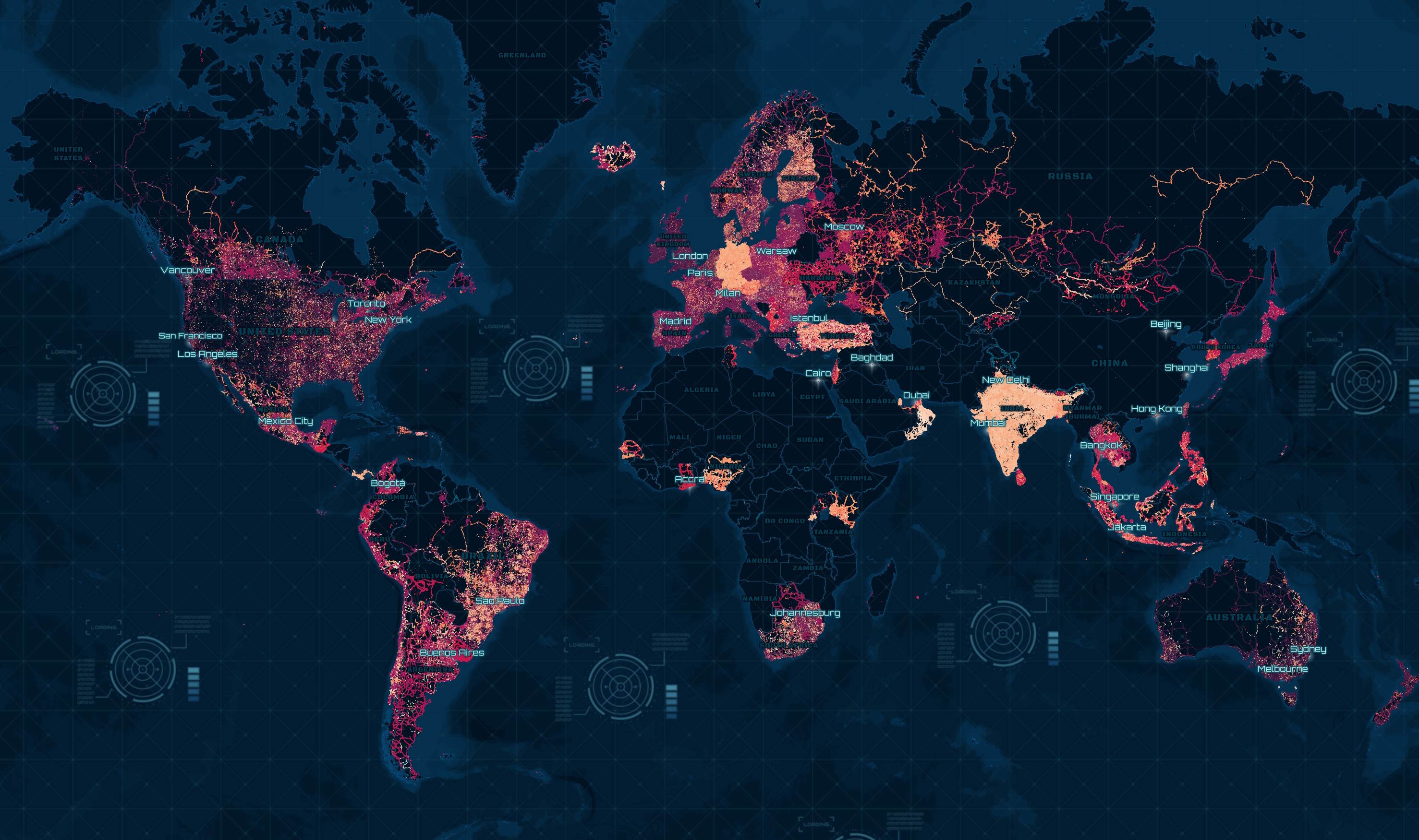
In this post, I'll convert this dataset into Parquet and examine its geospatial patterns.
My Workstation
I'm using a 5.7 GHz AMD Ryzen 9 9950X CPU. It has 16 cores and 32 threads and 1.2 MB of L1, 16 MB of L2 and 64 MB of L3 cache. It has a liquid cooler attached and is housed in a spacious, full-sized Cooler Master HAF 700 computer case.
The system has 96 GB of DDR5 RAM clocked at 4,800 MT/s and a 5th-generation, Crucial T700 4 TB NVMe M.2 SSD which can read at speeds up to 12,400 MB/s. There is a heatsink on the SSD to help keep its temperature down. This is my system's C drive.
The system is powered by a 1,200-watt, fully modular Corsair Power Supply and is sat on an ASRock X870E Nova 90 Motherboard.
I'm running Ubuntu 24 LTS via Microsoft's Ubuntu for Windows on Windows 11 Pro. In case you're wondering why I don't run a Linux-based desktop as my primary work environment, I'm still using an Nvidia GTX 1080 GPU which has better driver support on Windows and ArcGIS Pro only supports Windows natively.
Installing Prerequisites
I'll use DuckDB v1.4.3, along with its H3, JSON, Lindel, Parquet and Spatial extensions, in this post.
$ cd ~
$ wget -c https://github.com/duckdb/duckdb/releases/download/v1.4.3/duckdb_cli-linux-amd64.zip
$ unzip -j duckdb_cli-linux-amd64.zip
$ chmod +x duckdb
$ ~/duckdb
INSTALL h3 FROM community;
INSTALL lindel FROM community;
INSTALL json;
INSTALL parquet;
INSTALL spatial;
I'll set up DuckDB to load every installed extension each time it launches.
.timer on
.width 180
LOAD h3;
LOAD lindel;
LOAD json;
LOAD parquet;
LOAD spatial;
The maps in this post were rendered using QGIS version 3.44. QGIS is a desktop application that runs on Windows, macOS and Linux. The application has grown in popularity in recent years and has ~15M application launches from users all around the world each month.
I used QGIS' HCMGIS plugin to add basemaps from Esri to the maps in this post.
Downloading Emily's JSON Files
The following will download 131 JSON files which are 647 MB uncompressed. These files were last refreshed on December 4th.
$ mkdir -p ~/emily_biz
$ cd ~/emily_biz

$ wget -r -A json https://geo.emily.bz/coverage-dates
Below is an example record from one of the JSON files.
$ jq -S \
    .customCoordinates[0] \
    geo.emily.bz/coverage-dates/aland.json
{
  "extra": {
    "tags": [
      "2009-08"
    ]
  },
  "lat": 60.023421733271704,
  "lng": 20.58331925203021
}
Producing Parquet
Below, I'll create a table in DuckDB and import the data from the JSON files.
$ ~/duckdb street_view.duckdb
CREATE OR REPLACE TABLE street_view (
    geometry   GEOMETRY,
    updated_at DATE);
$ for FILENAME in geo.emily.bz/coverage-dates/*.json; do
      echo $FILENAME
      echo "
          INSERT INTO street_view
              WITH a AS (
                  SELECT UNNEST(customCoordinates) a
                  FROM   READ_JSON('$FILENAME'))
              SELECT geometry:   ST_POINT(a.lng, a.lat),
                     updated_at: (a.extra.tags[-1] || '-01')::DATE
              FROM   a
              WHERE  a.extra.tags[-1] LIKE '2%'" \
          | ~/duckdb street_view.duckdb
  done
I'll then export this table as a spatially-sorted, ZStandard-compressed Parquet file.
$ ~/duckdb street_view.duckdb
COPY (
    FROM     street_view
    ORDER BY HILBERT_ENCODE([ST_Y(ST_CENTROID(geometry)),
                             ST_X(ST_CENTROID(geometry))]::double[2])
) TO 'street_view.parquet' (
        FORMAT 'PARQUET',
        CODEC  'ZSTD',
        COMPRESSION_LEVEL 22,
        ROW_GROUP_SIZE 15000);
The resulting Parquet file is 85 MB and contains 7,163,407 rows.
Data for Bosnia and Herzegovina, Cyprus, Namibia, Paraguay and Vietnam are missing in this release. Hopefully, they will be available after the next refresh.
Data Fluency
Below are the point counts rounded up to the nearest thousand and broken down by year.
SELECT   year:  YEAR(updated_at),
         count: CEIL((COUNT(*) / 1000))::INT,
FROM     'street_view.parquet'
GROUP BY 1
ORDER BY 1;
┌───────┬───────┐
│ year  │ count │
│ int64 │ int32 │
├───────┼───────┤
│  2003 │     1 │
│  2006 │     1 │
│  2007 │    28 │
│  2008 │   251 │
│  2009 │   659 │
│  2010 │   344 │
│  2011 │   619 │
│  2012 │   792 │
│  2013 │   622 │
│  2014 │   474 │
│  2015 │   661 │
│  2016 │   529 │
│  2017 │    70 │
│  2018 │   142 │
│  2019 │   195 │
│  2020 │    50 │
│  2021 │   267 │
│  2022 │   507 │
│  2023 │   588 │
│  2024 │   290 │
│  2025 │    83 │
├───────┴───────┤
│    21 rows    │
└───────────────┘
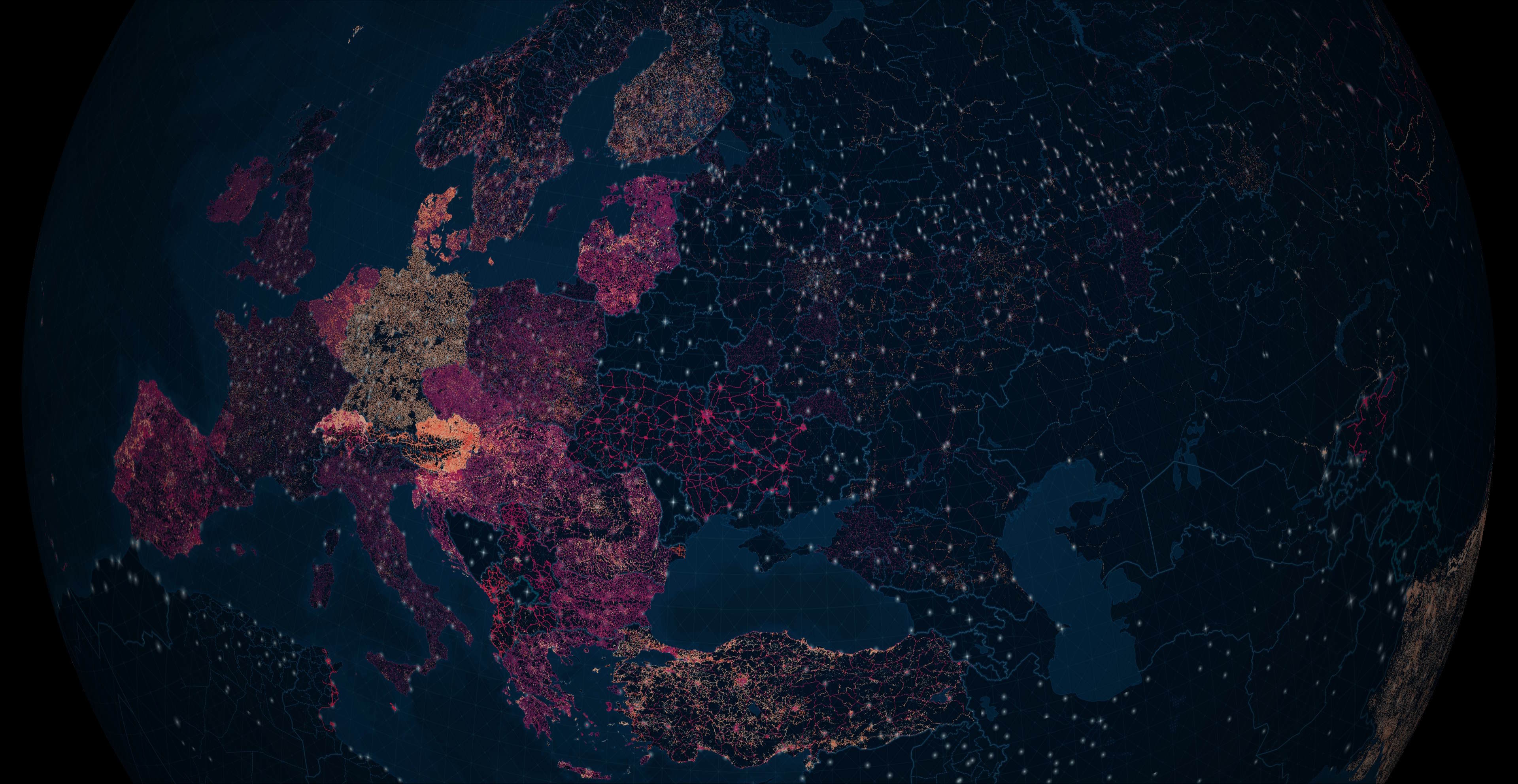
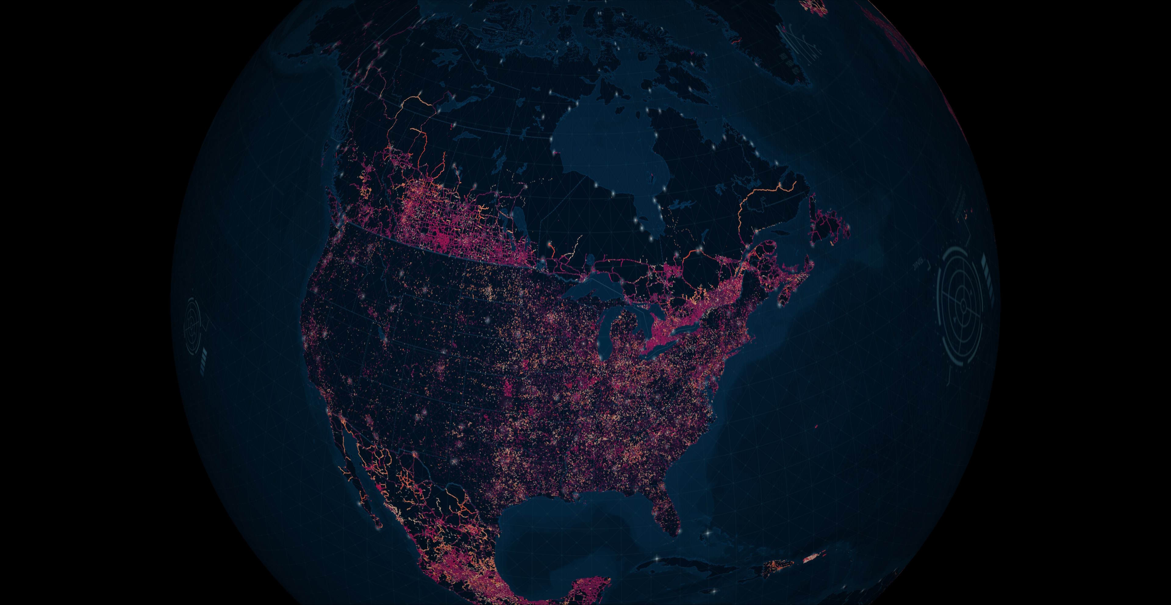
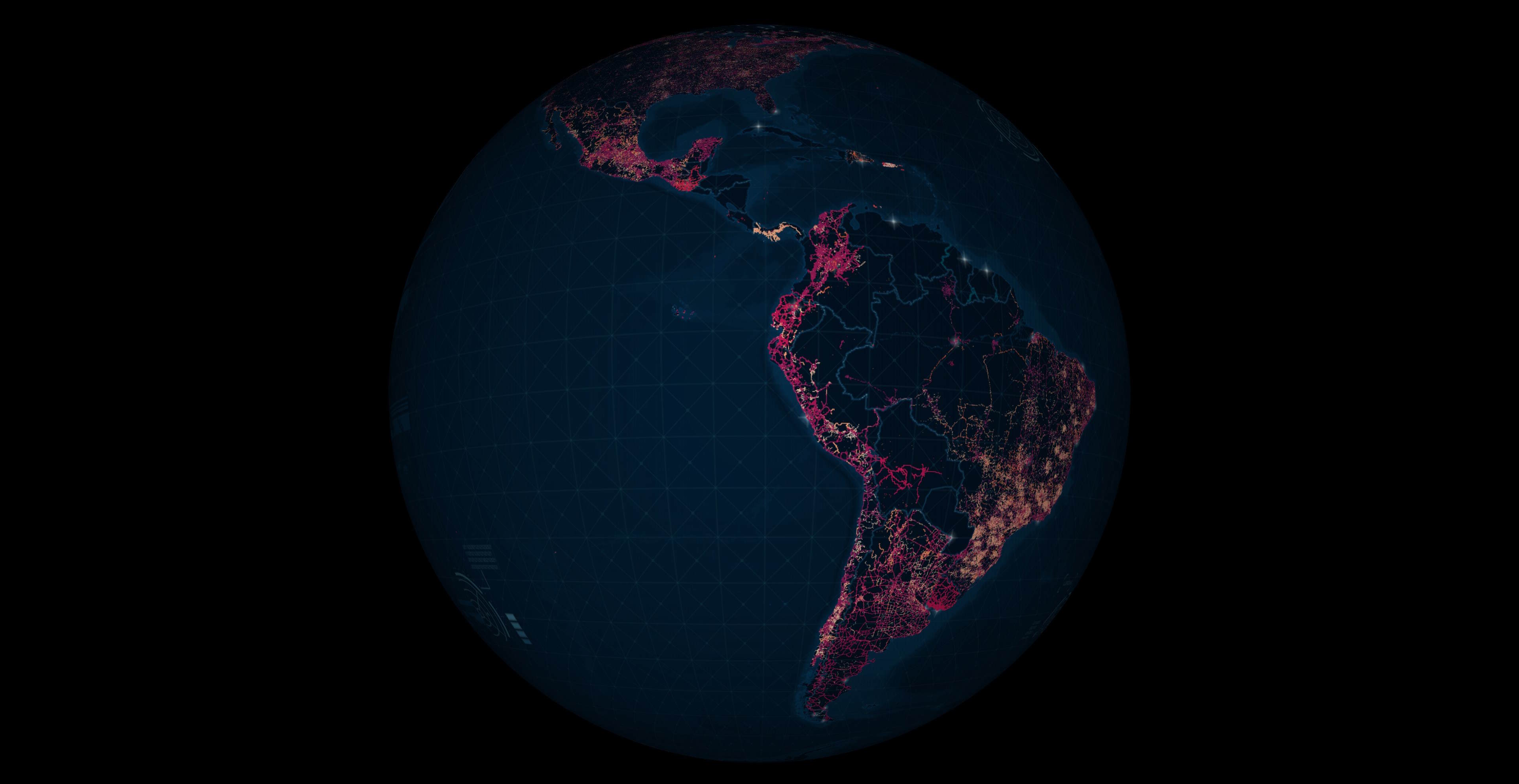
Below is the coverage across Europe. The darker colours are points that were updated closer to 2007 and the brighter colours closer to December of last year.
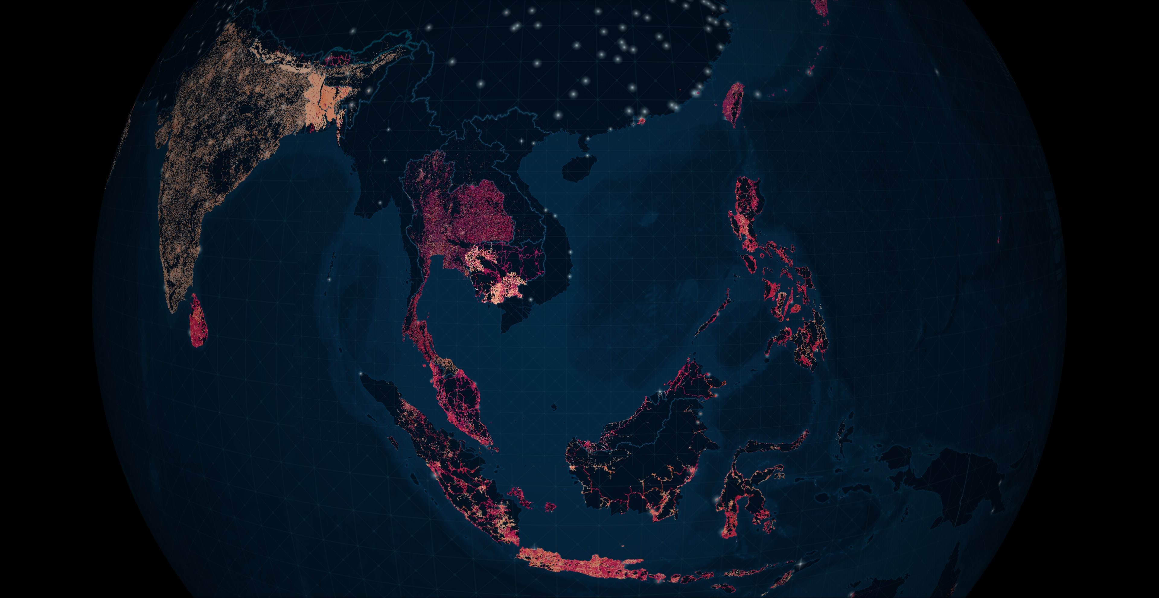
The following shows India and Southeast Asia's coverage.
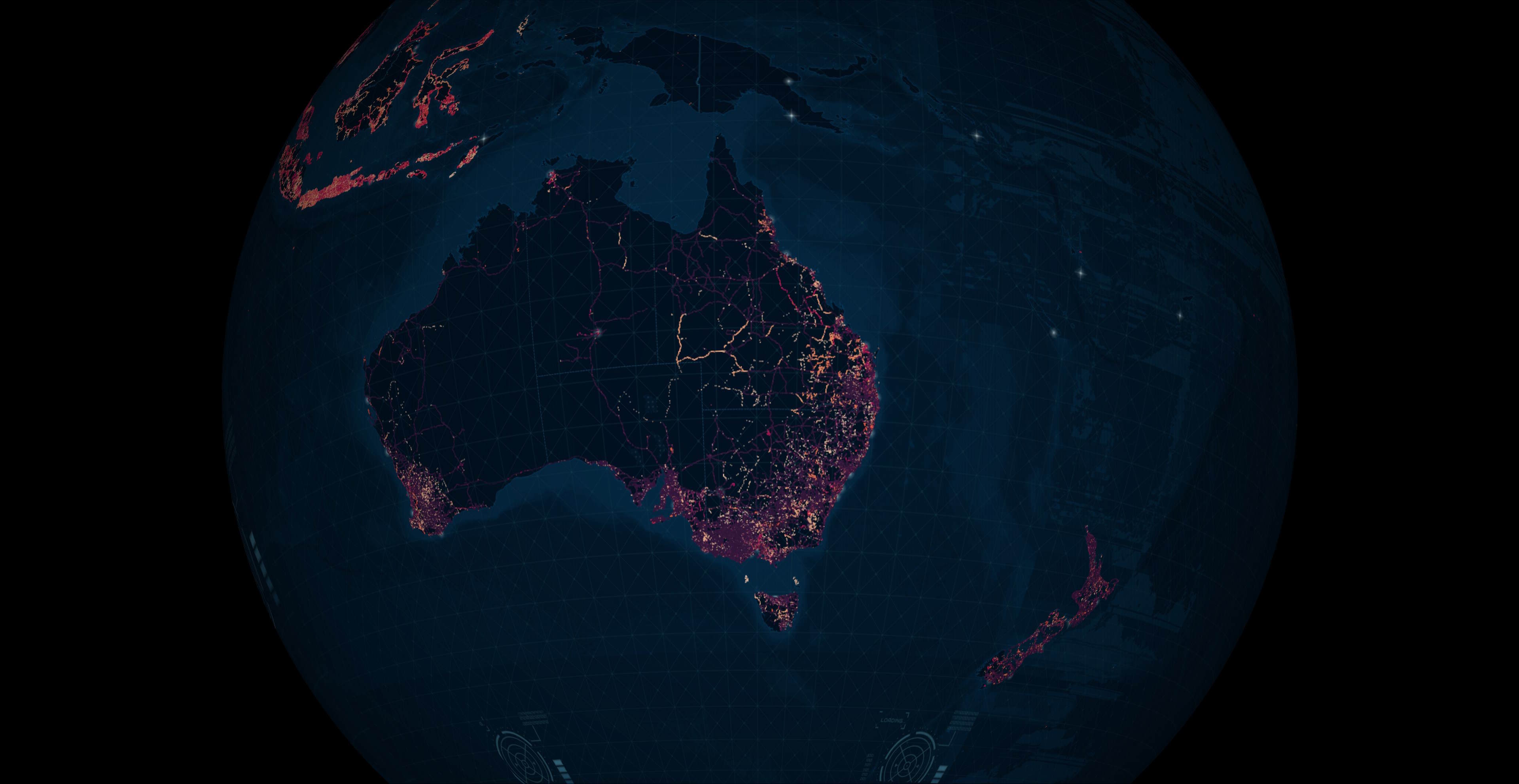
The following shows the coverage across Australia and New Zealand.
This is the coverage for North America.
This is the coverage for Latin America and the Caribbean.
Thank you for taking the time to read this post. I offer both consulting and hands-on development services to clients in North America and Europe. If you'd like to discuss how my offerings can help your business please contact me via LinkedIn.