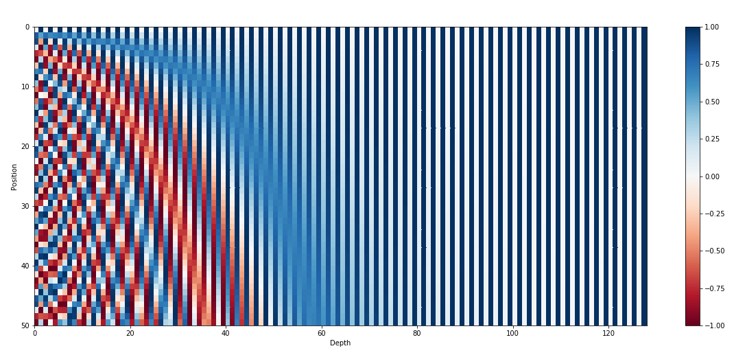
If the following image doesn’t make sense to you, there’s a good chance you haven’t fully grasped positional encodings in transformer architecture. Please stick around as I’ll try to explain them in a way that actually feels intuitive.
Context
This blog is a part of my quest to properly understand the transformer architecture. Previously, I tried to explain self-attention in my own way here. This is just a continuation trying to explain positional encoding. Also, as I mentioned in my previous blog, I’ve taken heavy inspiration (and learning) from this video, and if you know Hindi, I would genuinely suggest you to rather go over his playlist.
Some background
To understand what positional encodings are, lets zoom into this section of the transformer architecture
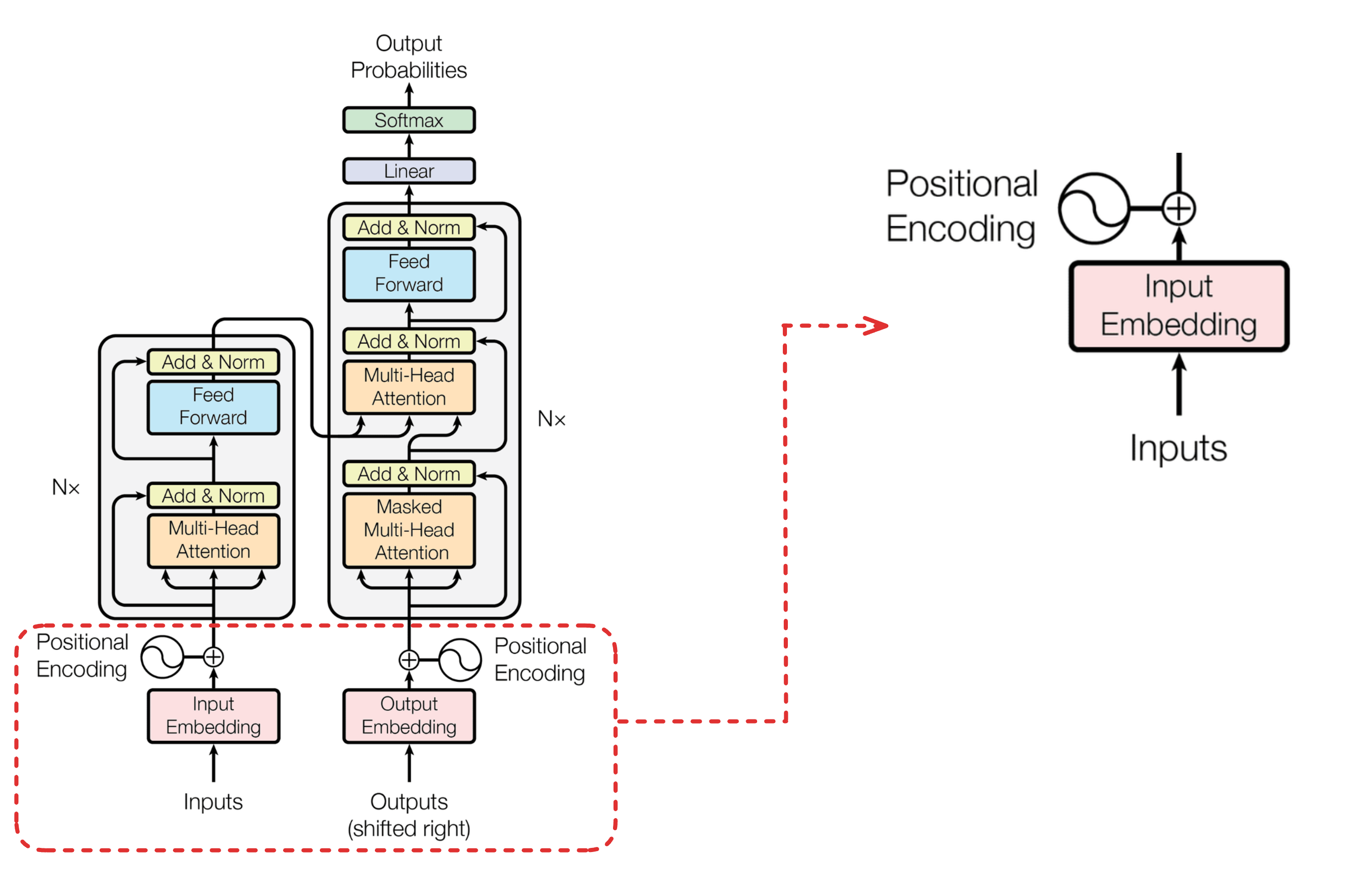
Now, lets break down the components you see in the zoomed-in figure.
Inputs
These are the words that are fed into the model. Before being fed, these words go through what’s called tokenization, a process that breaks text into smaller units called tokens. Tokenization is a vast field in itself, so I won’t be covering it in this blog. For simplicity, let’s assume each word in the English language has a unique ID associated with it. When we pass a sentence to a transformer, we are actually passing an array of these token IDs as input.
Input Embedding
The token IDs by themselves are just integers, i.e., they don’t carry any semantic meaning. The input embedding layer converts each token ID into a dense vector of fixed dimension (say, 512 or 768). Think of it as a lookup table: each token ID maps to a learnable vector that captures the meaning of that word. These vectors are what the transformer actually works with. Think of it like converting a single number into an n-dimensional vector that has semantic meaning.
Positional Encoding
The need
Now that we understand how an input sentence gets converted into dense vectors, let’s understand why we need positional encoding in the first place.
So far, we’ve converted a list of words into a list of dense vectors. But here’s the problem: the embedding for a word is always the same regardless of where it appears in the sentence. The word “love” will have the same vector whether it’s the first word or the last.
Consider: “I love transformers” vs “Transformers love I” (yeah you grammar nazis, the second one isn’t a grammatically valid sentence, but please bear with me to understand the concept). These two sentences have the exact same words, yet their meanings are completely different. The position of words matters! What if we could inject some positional information into each word’s embedding so that the same word at different positions gets a slightly different representation?
The simplest way
Let’s think from first principles. What’s the simplest way to add position information to a vector?
What if we just add the word’s index to its embedding? So the first word gets +0 added to all dimensions, the second word gets +1, the third gets +2, and so on. This would shift each word’s embedding based on its position in the sentence.

Simple, right? But there are some major issues with this approach:
Unbounded values: The number of input words can grow quite large (512, 1024, even 4096 tokens). If we keep adding the word’s index, the position values can become massive. Imagine adding 4096 to every dimension of a word embedding, the positional information would completely overpower the actual semantic meaning of the word.
Inconsistent scale: The first word gets +0, but the 1000th word gets +1000. This huge variation in magnitude makes it hard for the model to learn meaningful patterns.
So ok, then what if we normalize the index before adding it to the word embedding? That should get rid of the above issues right?
For example, we could divide the position by the total sequence length (N): position 0 becomes 0, position 1 becomes 1/N, position 2 becomes 2/N, and so on. This keeps all values between 0 and 1, so yeah, this kinda solves the above two issues.
But wait, this creates a new problem. The same word at the same absolute position would get different positional values depending on the sentence length! In a 10-word sentence, position 5 gets 0.5. In a 100-word sentence, position 5 gets 0.05. The model would have a hard time learning that these represent the “same” position.
Also, both approaches add discrete integers to the embedding. Neural networks generally work better with smooth, continuous representations rather than jumpy discrete values.
Another limitation of raw position indices is that they don’t naturally encode distance. The model knows absolute positions, but understanding how far apart two tokens are requires learning subtraction. Something like a periodic function could help here. Since it repeats its pattern after a fixed interval, shifting from position p to p + k results in a predictable transformation rather than a completely new value. This makes the relationship between positions easier to capture, allowing the model to learn relative distances through simple transformations instead of explicit arithmetic.
So to summarize this section, we need something that ticks all three boxes:
- Bounded: Values stay in a fixed range regardless of position
- Continuous: Smooth transitions between positions
- Periodic: Can encode relative distances naturally
Trigonometric Functions
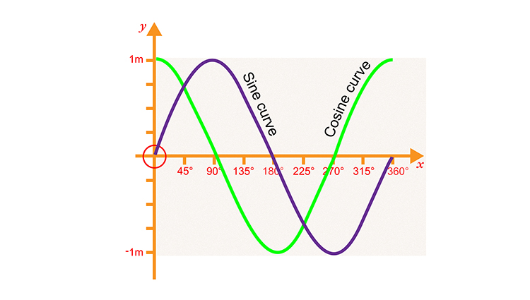
Enter sine and cosine, the perfect candidates! They’re bounded between -1 and 1, inherently continuous, and periodic.
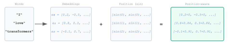
So let’s just add $\sin(\text{pos})$ to each word embedding: position 0 gets $\sin(0)$, position 1 gets $\sin(1)$, position 2 gets $\sin(2)$, and so on.
But there’s one big issue: each position needs a unique encoding. If two positions have the exact same encoding, the model will get confused and ambiguity is something we want to avoid in deep learning. Since sine is periodic, $\sin(n) = \sin(n + 2\pi)$, meaning different positions could end up with identical values.
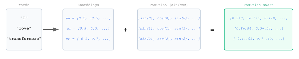
One way to counter this is to use two different trigonometric functions instead of one. What if we do:
$$y = y_{\text{emb}} + [\sin(\text{pos}), \cos(\text{pos}), \sin(\text{pos}), \cos(\text{pos}), \ldots]$$
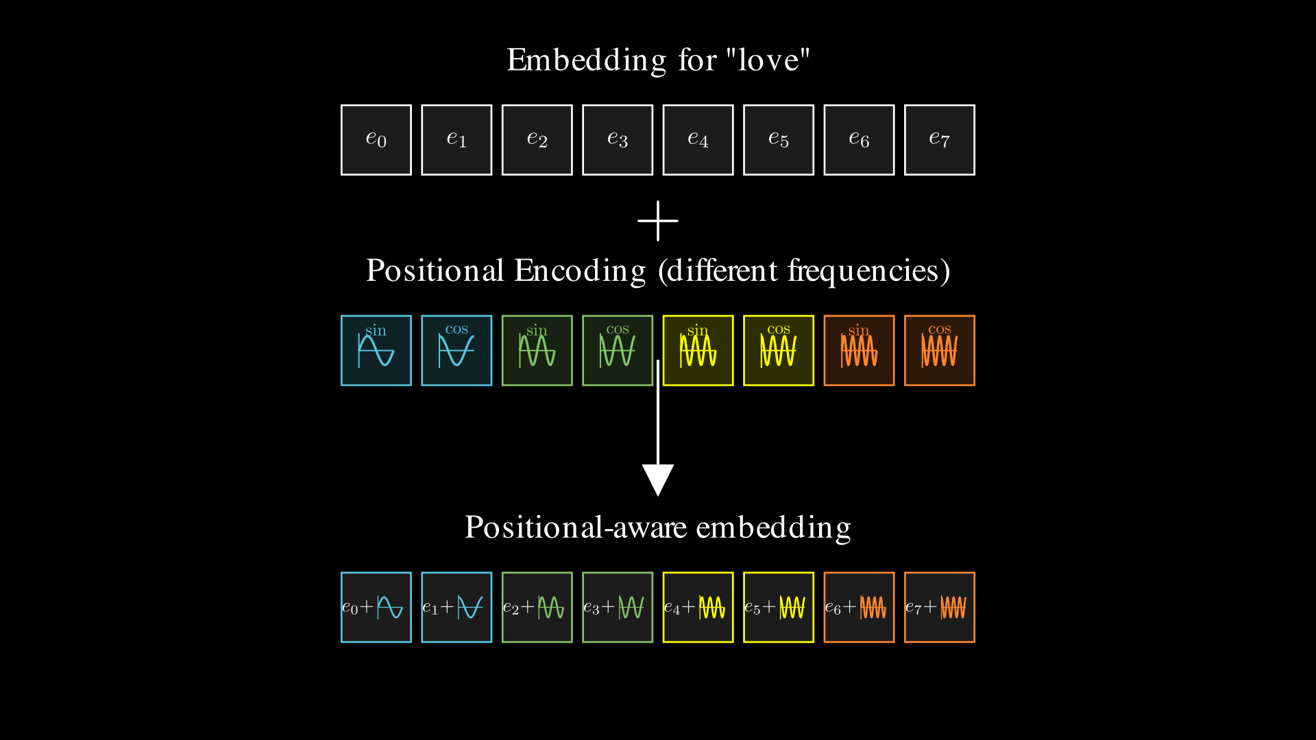
This helps in short sequences. But if the sequence is long enough, the values will eventually repeat, just like how a clock resets every 12 hours. To truly minmize chances of collision, we can make each dimension of the position encoding vector to use a different frequency for sine and cosine. That way, the pattern of values across all dimensions never (rarely) repeats within any reasonable sequence length.
So, instead of just $[\sin(\text{pos}), \cos(\text{pos}), \sin(\text{pos}), ...]$, we use:
$$[\sin(\omega_1 \cdot \text{pos}), \cos(\omega_1 \cdot \text{pos}), \sin(\omega_2 \cdot \text{pos}), \cos(\omega_2 \cdot \text{pos}), \ldots]$$
where each $\omega_k$ is a different frequency for each dimension. This way, every position gets a unique, high-dimensional fingerprint that’s extremely unlikely to repeat or collide with any other position.
Take a minute to pause and reflect on the figure below, this should give you a very good intuition as to what exactly positional encoding is doing.
The Formula
If you are clear about the things we talked earlier, its finally time to introduce the famous/dearding positional encoding formula from the original Transformer paper:
$$PE_{(pos, 2i)} = \sin\left(\frac{pos}{10000^{2i/d_{model}}}\right)$$ $$PE_{(pos, 2i+1)} = \cos\left(\frac{pos}{10000^{2i/d_{model}}}\right)$$
Where:
- $pos$ is the position of the word in the sequence
- $i$ is the dimension index
- $d_{model}$ is the embedding dimension (e.g., 512)
The key to understanding this formula lies in the frequency term
$$\frac{1}{10000^{2i/d_{model}}}$$
It may look intimidating at first, but it’s really doing just one simple thing: assigning a different frequency to each pair of dimensions.
Instead of every dimension using the same sine or cosine wave, each dimension oscillates at a different frequency that depends on the dimension index.
At the starting dimensions, the frequency of the sine and cosine waves is very high, meaning the values change rapidly as the position increases. As we gradually move toward higher dimensions, the frequency becomes lower and lower, so the waves change much more slowly with position.
This is exactly what you saw in the first figure of the blog:
- Early dimensions (small (i)) → high-frequency waves → rapid oscillations across positions
- Later dimensions (large (i)) → low-frequency waves → slow, smooth changes across positions
So the left side of the heatmap looks dense and stripy, while the right side looks smoother and more gradual, all because the frequency decreases as we move across dimensions.
I visualized this heatmap using Manim (vibe-coded with Gemini 3, credit where its due!), and the result is quite satisfying to watch.
To conclude, in simple terms: the the positional encoding just alternates sine and cosine waves with different frequencies across the dimensions of the positional vector, scaled by the token’s position.