The Strait of Hormuz has experienced five major disruption episodes since 1981, ranging from a multi-year tanker war to brief seizure incidents. With the current 2026 conflict disrupting commercial traffic through the strait, a natural question arises: how long should we expect this disruption to last?
This analysis fits an exponential duration model to the observed episodes, treating the ongoing 2026 disruption as right-censored, and produces distributional forecasts for remaining duration.
The Dataset
Five episodes were identified through open-source reporting. Each has a clearly defined onset; four have resolved and one (the 2026 conflict) is ongoing as of the observation date.
| Episode | Start | End / Cutoff | Duration (d) | Status |
|---|---|---|---|---|
| Tanker War | 1981-05-01 | 1988-08-04 | 2,652 | Resolved |
| 2019 Shipping Crisis | 2019-05-12 | 2019-09-27 | 138 | Resolved |
| Advantage Sweet Detention | 2023-04-27 | 2024-07-11 | 441 | Resolved |
| St Nikolas Detention | 2024-01-11 | 2026-01-12 | 732 | Resolved |
| 2026 Conflict | 2026-02-28 | 2026-03-08 | 8+ | Ongoing ⏳ |
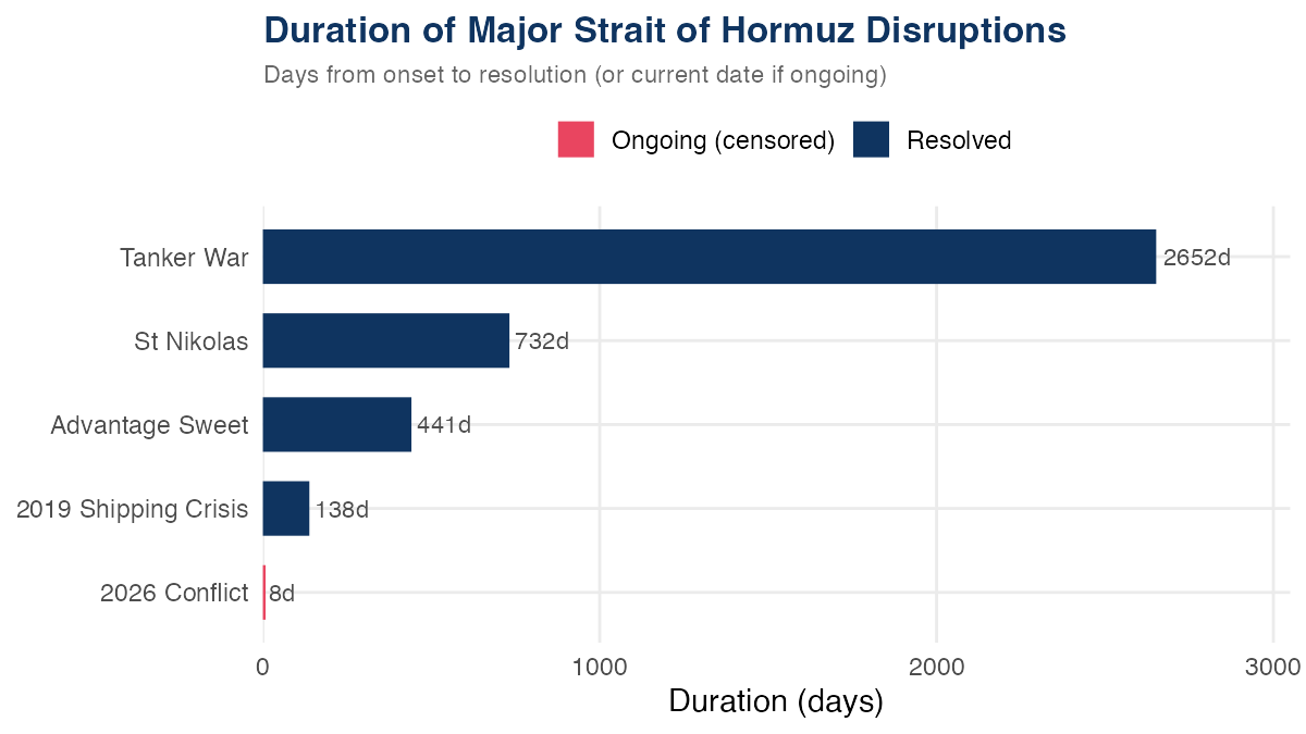
Figure 1. Duration of each episode in days. The 2026 conflict (red) is ongoing and right-censored at 8 days.
Model Selection
The natural candidates for duration data are:
- Exponential — constant hazard rate (memoryless)
- Weibull — allows for increasing or decreasing hazard
- Generalized Gamma — nests both Weibull and log-normal
I considered all three. The Weibull shape parameter estimated near 1.0, which reduces the Weibull to an exponential. The generalized gamma was numerically unstable on this sample — unsurprising given just 4 observed events drawn from heterogeneous geopolitical regimes. The exponential is the appropriate choice: it has one parameter to estimate from minimal data, and a useful memorylessness property for forecasting.
Exponential Duration Model
Under the exponential model, the duration T of a disruption episode follows:
T ~ Exp(λ)
S(t) = P(T > t) = exp(−λt)
E[T] = 1/λ Median[T] = ln(2)/λ
With right-censored data, the MLE for λ is simply:
λ̂ = d / Σ tᵢ
where d = 4 is the number of observed (resolved) events and Σ tᵢ = 3,971 is total exposure across all five episodes. This gives:
The 95% confidence interval for λ, based on the exact Poisson method with 4 observed events, is (0.000274, 0.002577) per day. This translates to a mean duration range of roughly 388 to 3,650 days — reflecting substantial uncertainty with only four resolved episodes.
Fitted Survival Curve
The fitted survival function shows the probability that a disruption episode is still ongoing at time t. Observed durations are plotted as points:
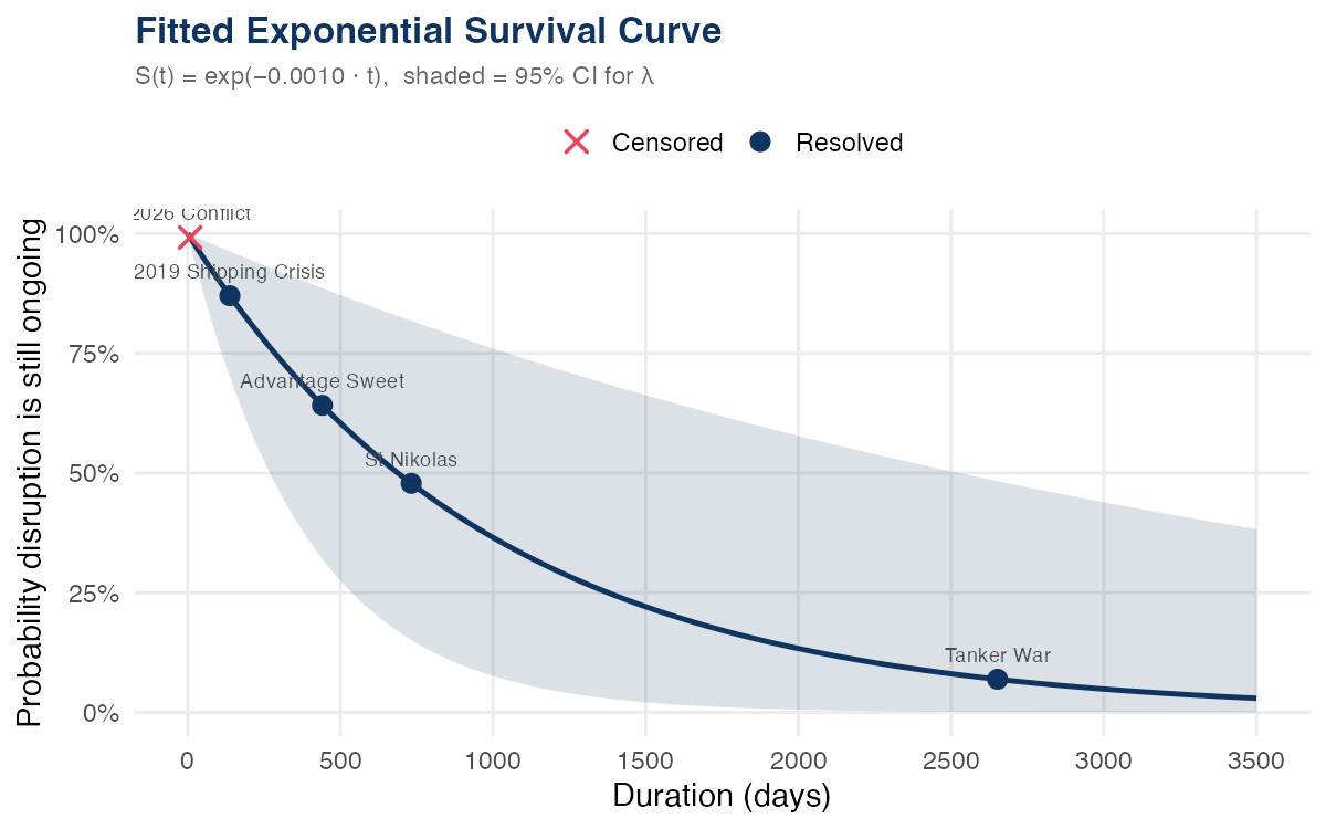
Figure 2. Exponential survival curve with 95% CI band. Circles are resolved episodes; the × is the 2026 conflict (right-censored at 8 days).
The Tanker War, at 2,652 days, falls in the far right tail — a low-probability but historically realized outcome. The 2019 crisis, at just 138 days, resolved while the survival probability was still above 85%.
Forecasting the Current Episode's Remaining Duration
A key property of the exponential distribution is memorylessness:
P(T > t + s | T > t) = P(T > s)
This means that given the disruption has already lasted 8 days, the conditional distribution of remaining duration is the same exponential distribution as if it had just started. The forecast does not depend on how long the episode has already lasted.
Remaining Duration Forecast (from today)
Expected
993 days
~2.7 years
Median
688 days
~1.9 years
90th Percentile
2,286 days
~6.3 years
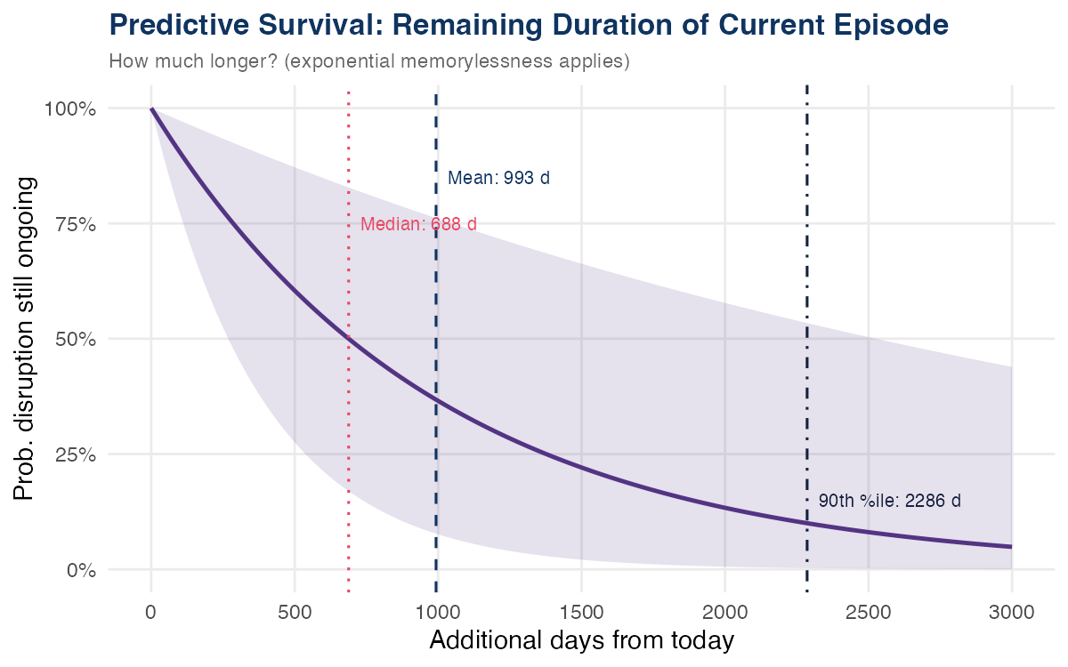
Figure 3. Predictive survival curve for the remaining duration of the 2026 disruption. Dashed lines mark the mean, median, and 90th percentile. Band shows 95% CI.
Put differently: the model gives a 50% probability that the current disruption resolves within about 1.9 years, but a 10% probability it persists beyond 6.3 years. The right tail is heavy.
Uncertainty
With only 4 observed events, parameter uncertainty is substantial. The figure below shows 95% confidence intervals for the key duration quantities:
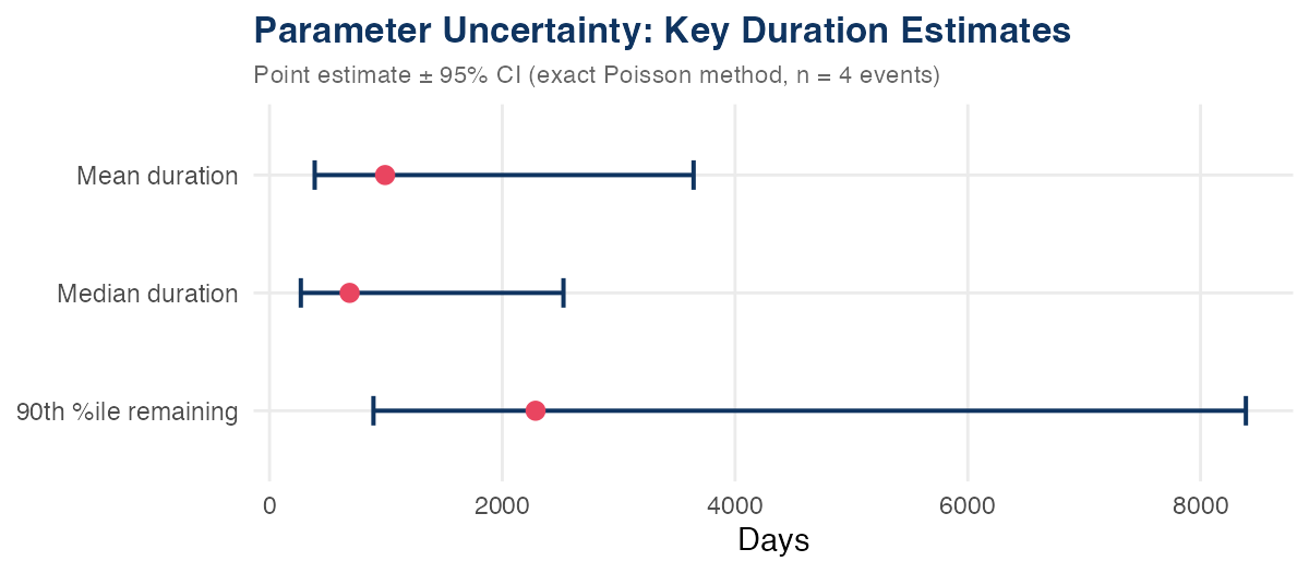
Figure 4. Point estimates and 95% CIs for key duration quantities (exact Poisson method).
Extending the Model for Policy Reversal Risk
The baseline exponential model treats all Hormuz disruptions as drawn from a single process. But the current episode unfolds against a specific political backdrop in which there is meaningful — and repeatedly demonstrated — scope for rapid policy reversal. Market participants sometimes use the shorthand "TACO" to describe a pattern of threat-then-retreat behavior. Translating this into formal language: there may be a material de-escalation probability that the baseline Hormuz model, calibrated on historical disruptions, does not capture.
To address this, I construct a two-component mixture model. The idea is not to claim that tariff decisions and military escalation are the same process — they plainly are not. Rather, I use an observed sample of major tariff-escalation decisions and their time-to-retreat as a practical calibration device for a de-escalation branch in the disruption forecast.
Calibration Dataset: Major Tariff Decisions
Eleven major tariff-escalation decisions from 2025–2026 were coded, tracking the time from hard commitment or public threat to the first clear pause, rollback, or materially softer settlement. Episodes without a clear retreat by March 8, 2026 are right-censored.
| Episode | Days | Retreat? | ≤ 30d? |
|---|---|---|---|
| Canada/Mexico tariffs announced | 2 | ✓ | ✓ |
| Canada/Mexico tariffs reimposed | 3 | ✓ | ✓ |
| Canada steel 50% threat | 0.5 | ✓ | ✓ |
| Reciprocal tariffs pause | 7 | ✓ | ✓ |
| China 145% to truce | 33 | ✓ | |
| EU 50% threat delayed | 2 | ✓ | ✓ |
| Steel/aluminum 50% hike | 278+ | ||
| Mexico 30% threat paused | 19 | ✓ | ✓ |
| EU 30% threat to framework | 40 | ✓ | |
| Timber/furniture duties | 159+ | ||
| AI chip tariffs | 53+ |
Of the 11 episodes, 8 showed a clear retreat or softer settlement; 6 of those retreats occurred within 30 days. Three episodes remain unresolved.
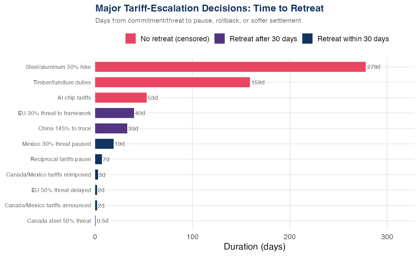
Figure 5. Time from tariff commitment to retreat, by episode. Red bars are censored (no retreat observed).
Mixture Specification
Define a two-component mixture for the remaining duration T of the current Hormuz disruption:
S(t) = p · exp(−λD · t) + (1 − p) · exp(−λH · t)
where:
- λH = 0.001007 / day — the baseline Hormuz hazard, estimated above
- λD = 1 / 5.58 ≈ 0.1791 / day — the de-escalation hazard, calibrated from the mean duration of the 6 within-30-day tariff retreats (2, 3, 0.5, 7, 2, 19 days)
- p = 6/11 ≈ 0.545 — the de-escalation probability, set to the observed share of tariff decisions with retreat within 30 days
A note on memorylessness: each component is exponential and therefore memoryless individually. However, the mixture itself is not memoryless. As time passes without resolution, the posterior weight on the de-escalation branch declines — the mixture "learns" that the quick-exit scenario has become less likely. This is a feature, not a bug: the mixture reflects latent regime uncertainty, where one branch represents rapid policy retreat and the other represents ordinary historical disruption persistence.
Mixture Results
Mixture Forecast: Remaining Duration
Expected
454 days
~1.2 years
90th Percentile
1,504 days
~4.1 years
95th Percentile
2,192 days
~6.0 years
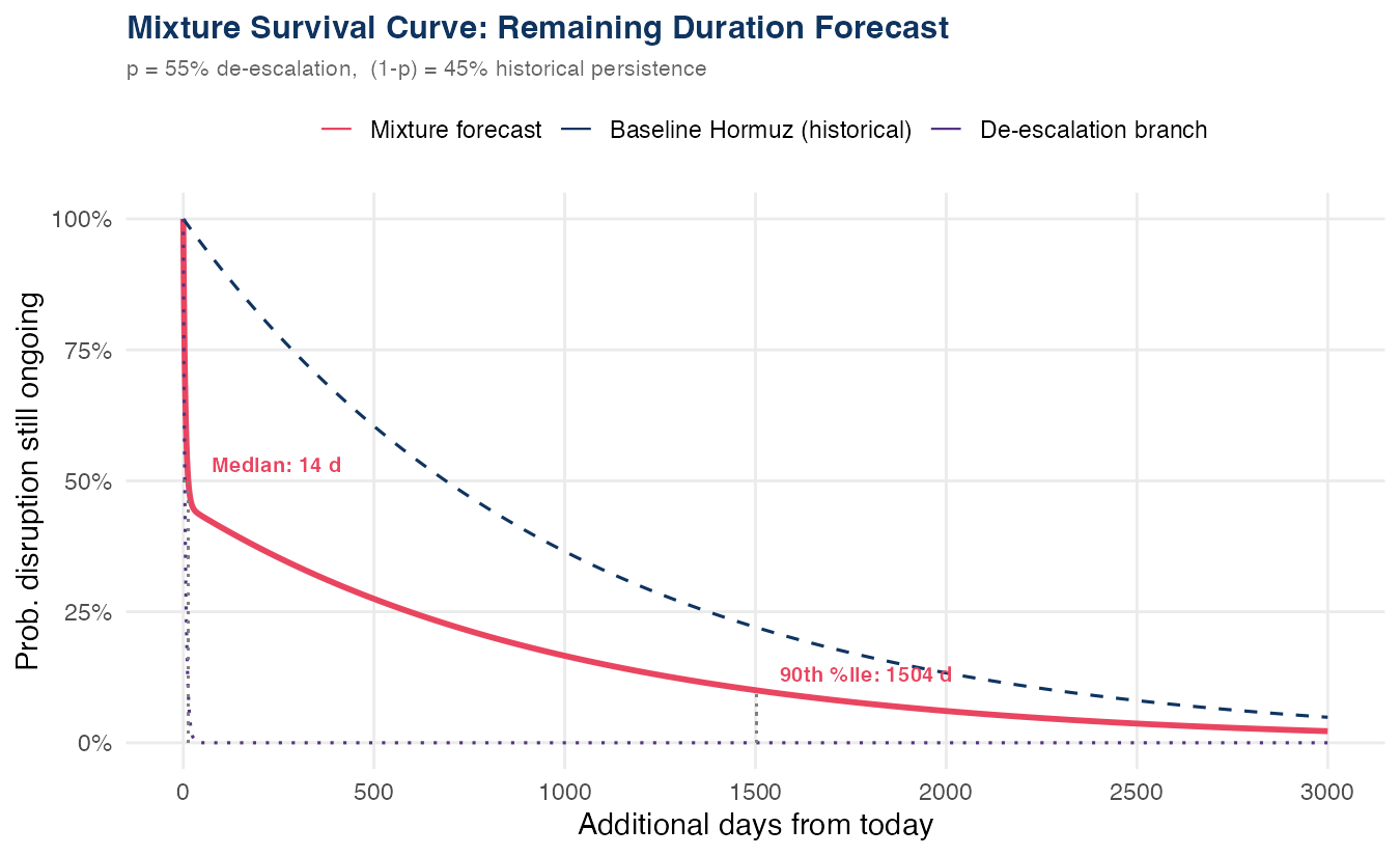
Figure 6. Mixture survival curve (solid red) with baseline Hormuz (dashed blue) and de-escalation branch (dotted purple). Annotated with mixture median and 90th percentile.
Interpretation
The mixture model produces a striking pattern: the median drops sharply from 688 days (baseline) to just 13 days, because the model now places roughly 55% probability on a rapid de-escalation branch. Yet the mean remains large at 454 days, because the broader-conflict branch still contributes a long right tail.
This is a classic mixture-distribution pattern: a lot of probability mass near "soon," but still meaningful weight on a prolonged episode. If the de-escalation branch is roughly right, there is a fair chance the disruption resolves quickly. If it does not, the remaining duration reverts toward the baseline Hormuz profile — and the right tail is long.
Sensitivity to De-escalation Probability
The main specification uses p = 6/11 ≈ 0.545, counting only retreats within 30 days. An alternative calibration uses p = 8/11 ≈ 0.727, counting any observed retreat by end of follow-up (not only those within 30 days). This more aggressive de-escalation assumption yields:
| Quantity | Main (p = 55%) | Alternative (p = 73%) |
|---|---|---|
| Mean remaining | 454 days | ~280 days |
| Median remaining | 13 days | ~15 days |
| 90th percentile | 1,504 days | ~996 days |
The 30-day calibration is preferred for the main specification, because the substantive question is about near-term climbdown — whether the current posture is likely to be walked back quickly — rather than eventual softening over many months.
Mixture Model Caveats
- Domain transfer. Tariff decisions and military/diplomatic crises are different processes. The tariff-retreat dataset is used as a calibration device for the de-escalation probability, not as proof that the two domains share a generating process.
- Conditional scenario. The mixture forecast is a scenario overlay on top of the baseline Hormuz model. It answers: "what changes if one allows for a material probability of rapid policy reversal?"
- Not structural. The model does not identify the mechanism by which de-escalation would occur. It quantifies the implication of assuming it might.
- Baseline remains primary. The historical Hormuz exponential model remains the baseline descriptive model. The mixture is an extension, not a replacement.
Why Reopening Can Lag De-escalation
The models above estimate the time until a political or military off-ramp. But a government decision to de-escalate is not the same thing as commercial normalization of shipping through the Strait of Hormuz. Even after a ceasefire, formal agreement, or diplomatic climbdown, shipping may remain impaired because:
- War-risk insurance may remain unavailable or prohibitively expensive; underwriters re-enter cautiously after withdrawal.
- Shipowners may refuse to sail without credible security guarantees, regardless of government pronouncements.
- Escort arrangements (naval convoys, demining) take time to organize and deploy.
- Residual threats — uncleared ordnance, rogue actors, or incomplete ceasefire compliance — may persist.
- Backlog clearing: as of early March 2026, Reuters reported approximately 150 vessels stranded or anchored near the chokepoint. Clearing this queue takes time even under ideal conditions.
A political decision to de-escalate would not automatically restore commercial transit through Hormuz. Shipping would still depend on war-risk insurance, security guarantees, vessel-owner willingness, and the clearing or management of residual threats. Historical and contemporary analogues suggest that formal agreement and functional reopening can be separated by days, weeks, or longer — so the forecast adds a reopening-lag component on top of the political-duration model.
This motivates a two-stage decomposition:
Ttotal = Tofframp + Treopen
where Tofframp is the time until a meaningful political/military off-ramp (estimated by the mixture model above), and Treopen is the additional operational lag until shipping actually resumes at a meaningful level.
Dataset A: Current Hormuz Operational State
The following daily panel tracks operational indicators from the onset of the 2026 disruption through the current observation date. It is assembled from public reporting (primarily Reuters) rather than an official administrative dataset. Some fields are sparse and event-driven rather than fully observed every day.
| Date | Tanker Transits |
Anchored Vessels |
War-Risk Premium |
Insurance | Escort | Attack 48h? |
Milestone | Traffic Norm% |
|---|---|---|---|---|---|---|---|---|
| Feb 28 | ~25 | ~20 | — | normal | none | Y | closed | ~100% |
| Mar 1 | ≤ 5 | ~40 | — | repriced | none | Y | closed | ~20% |
| Mar 2 | ≤ 3 | ~60 | — | partially withdrawn | none | Y | closed | ~12% |
| Mar 3 | ≤ 2 | ~80 | — | withdrawn | none | Y | closed | ~8% |
| Mar 4 | ≤ 2 | ~100 | — | withdrawn | none | Y | closed | ~8% |
| Mar 5 | ≤ 2 | ~120 | — | withdrawn | proposed | closed | ~8% | |
| Mar 6 | ≤ 2 | ~130 | — | withdrawn | proposed | Y | closed | ~8% |
| Mar 7 | ≤ 2 | ~140 | — | withdrawn | announced | closed | ~8% | |
| Mar 8 | ≤ 2 | ~150 | — | gov’t backstop announced | announced | closed | ~8% |
Dataset A. Daily operational panel assembled from public reporting (primarily Reuters). Pre-war baseline: ~25 tanker transits/day. Some counts are interpolated between confirmed reports. War-risk premium data not available at daily granularity; — = not reported that day.
Dataset A matters because it tracks reopening as an operational process, not just a diplomatic event. As of March 8, traffic normalization stands at roughly 8% of baseline, with ~150 vessels stationary, insurance withdrawn, and the U.S. reinsurance/escort program only at the "announced" stage. Even an immediate ceasefire would leave substantial ground to cover.
Dataset B: Shipping-Reopening Analogues
To calibrate the reopening lag, I draw on maritime analogues where a formal agreement or de-escalation signal preceded the resumption of commercial shipping. These are not identical processes — they are externally grounded calibration points.
| Analogue | Agreement | First Transit | Lag (d) | Notes |
|---|---|---|---|---|
| Black Sea grain corridor | 2022-07-22 | 2022-08-01 | ~10 | Insurers required escort/mine-management before cover |
| Red Sea post-ceasefire | 2025 (qual.) | — | weeks–months | Shipping execs said ceasefire would not immediately restore traffic |
| Hormuz 2026 (official est.) | — | — | weeks | Reuters-reported U.S. official expectation for stabilization |
Reopening-Lag Model
Rather than fitting a parametric model to these few data points, I use a discrete scenario distribution for Treopen, motivated by the analogues:
| Scenario | Range | Weight | Motivation |
|---|---|---|---|
| Short | 7–14 days | 30% | ~10-day Black Sea precedent; strong U.S. backstop |
| Medium | 21–45 days | 50% | Reuters “weeks” guidance; insurance re-entry lag |
| Long | 60–120 days | 20% | Red Sea analogue; residual threats; slow insurer re-entry |
Within each scenario, Treopen is drawn uniformly over the range. The expected reopening lag is 0.30 × 10.5 + 0.50 × 33 + 0.20 × 90 ≈ 38 days.
Combined Two-Stage Forecast
The combined forecast is computed by Monte Carlo simulation (200,000 draws): sample Tofframp from the mixture model, then independently sample Treopen from the scenario distribution, and add them.
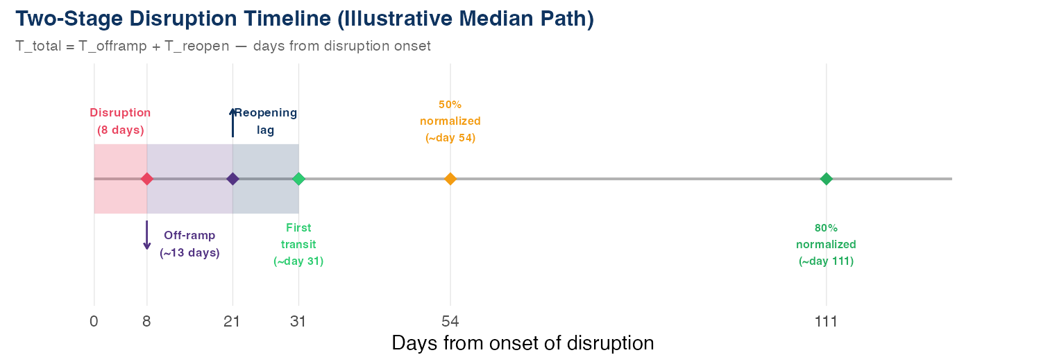
Figure 7. Illustrative median-path timeline for the two-stage model. The off-ramp and reopening phases are sequential; normalization milestones follow.
Full Two-Stage Forecast: Time to Meaningful Transit
Expected
489 days
~1.3 years
90th Percentile
1,531 days
~4.2 years
Compare these to the mixture-only forecast (which assumes instant reopening upon de-escalation): that model’s median was 13 days. Adding the operational reopening lag shifts the median from 13 days to 88 days — a roughly 6× increase. The mean shifts from 454 to 489 days, and the 90th percentile from 1,504 to 1,531 days. The right tail is dominated by Stage 1 (long-duration conflict), so the reopening lag matters most in the short-to-medium horizon.
Probability of Reopening Within Key Horizons
| Question | Probability |
|---|---|
| Meaningful transit resumes within 14 days? | ~7% |
| Meaningful transit resumes within 30 days? | ~21% |
| Meaningful transit resumes within 90 days? | ~51% |
| Traffic still materially impaired after 60 days? | ~56% |
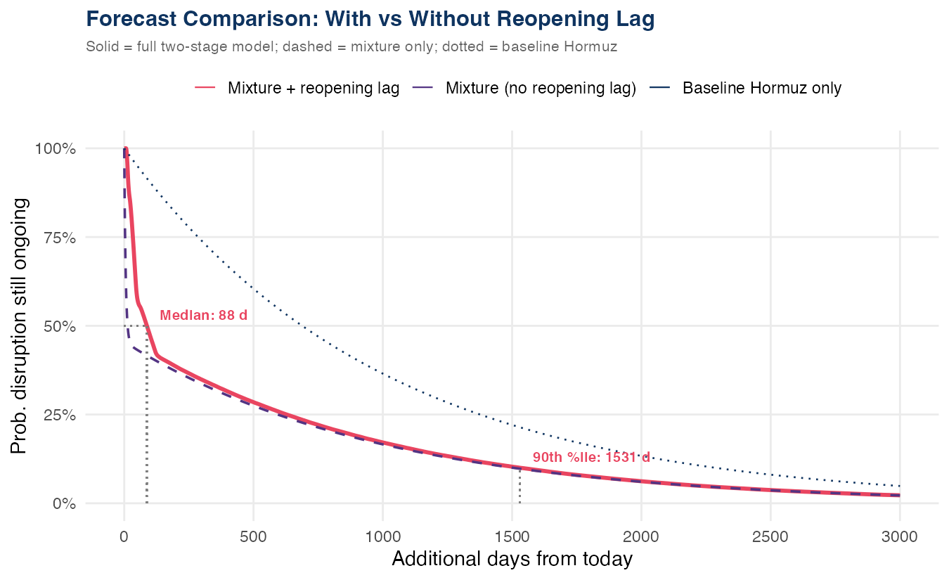
Figure 8. Forecast comparison: solid red = full two-stage model (mixture + reopening lag), dashed purple = mixture only (instant reopening), dotted blue = baseline Hormuz only.
Reopening-Lag Caveats
- Scenario-based, not estimated. The reopening-lag distribution is constructed from analogues and reporting, not fitted to a large sample.
- Independence assumption. Tofframp and Treopen are treated as independent. In practice, a longer conflict might also produce a longer reopening lag (e.g., more damage to clear).
- Analogue limits. The Black Sea grain corridor and Red Sea are different waterways with different threat profiles, insurance markets, and naval commitments.
- Not a forecast of normalization. This layer estimates time to first meaningful transit, not full normalization to pre-war levels. Full normalization could take substantially longer.
Limitations
All three model layers are descriptive, not structural. Key caveats:
- Tiny samples. The Hormuz model has n = 5 episodes (4 observed); the tariff calibration uses 11 decisions; the reopening-lag layer draws on 2–3 analogues. Uncertainty is substantial at every stage.
- Episode heterogeneity. The Tanker War (a multi-year interstate conflict) and the 2019 tanker seizures (a diplomatic incident) are qualitatively different events. Pooling them assumes a common generating process.
- Hand-curated boundaries. Episode start and end dates involve editorial judgment. Alternative definitions would shift the estimates.
- Constant hazard assumption. Each exponential component assumes no time-dependence in the probability of resolution — a simplification.
- Not causal. None of these models captures the geopolitical mechanics that determine when a disruption ends or shipping resumes.
- Cross-domain calibration. Using tariff-retreat patterns to calibrate a military de-escalation branch, and Black Sea/Red Sea analogues to calibrate Hormuz reopening, requires accepting that behavioral patterns transfer — strong assumptions stated explicitly throughout.
Conclusion
The baseline exponential model fitted to five major Strait of Hormuz disruptions estimates a mean episode duration of approximately 993 days (median 688 days). Under the memorylessness property, these figures also apply to the forecasted remaining duration of the current 2026 conflict.
The mixture extension, calibrated to an observed pattern of rapid policy reversal in tariff decisions, compresses the median political de-escalation forecast to roughly 13 days — reflecting a 55% probability of quick de-escalation — while the mean remains at 454 days because the broader-conflict tail is long.
Adding a reopening-lag layer — recognizing that a political decision to de-escalate does not immediately restore commercial shipping — shifts the median forecast for meaningful transit resumption to approximately 88 days (~3 months), with a mean of 489 days. There is roughly a 21% probability of meaningful transit within 30 days, but a 56% probability that traffic remains materially impaired after 60 days.
All three layers carry wide uncertainty. The baseline is a statistical summary of historical base rates. The mixture is a conditional scenario for policy reversal risk. The reopening lag is an operationally grounded extension informed by maritime analogues and current reporting. Together, they provide a structured framework for thinking about the range of plausible outcomes — not a point prediction.
Methodology: Baseline: Exponential MLE with right censoring, λ̂ = d / Σtᵢ, CIs via exact Poisson method. Mixture: two-component exponential mixture S(t) = p·exp(−λDt) + (1−p)·exp(−λHt), with p = 6/11 calibrated from 30-day tariff-retreat rates and λD = 1/5.58. Reopening lag: three-scenario uniform mixture (7–14d @ 30%, 21–45d @ 50%, 60–120d @ 20%), calibrated from Black Sea grain corridor, Red Sea expectations, and Reuters Hormuz reporting. Combined forecast via Monte Carlo convolution (200,000 draws). Observation date: March 8, 2026.