Next: Introduction [Contents][Index]
UNU.RAN – Universal Non-Uniform RANdom number generators
UNU.RAN (Universal Non-Uniform RAndom Number generator) is a collection of algorithms for generating non-uniform pseudorandom variates as a library of C functions designed and implemented by the ARVAG (Automatic Random VAriate Generation) project group in Vienna, and released under the GNU Public License (GPL). It is especially designed for such situations where
- a non-standard distribution or a truncated distribution is needed.
- experiments with different types of distributions are made.
- random variates for variance reduction techniques are used.
- fast generators of predictable quality are necessary.
Of course it is also well suited for standard distributions. However due to its more sophisticated programming interface it might not be as easy to use if you only look for a generator for the standard normal distribution. (Although UNU.RAN provides generators that are superior in many aspects to those found in quite a number of other libraries.)
UNU.RAN implements several methods for generating random numbers. The choice depends primary on the information about the distribution can be provided and – if the user is familar with the different methods – on the preferences of the user.
The design goals of UNU.RAN are to provide reliable, portable and robust (as far as this is possible) functions with a consisent and easy to use interface. It is suitable for all situation where experiments with different distributions including non-standard distributions. For example it is no problem to replace the normal distribution by an empirical distribution in a model.
Since originally designed as a library for so called black-box or universal algorithms its interface is different from other libraries. (Nevertheless it also contains special generators for standard distributions.) It does not provide subroutines for random variate generation for particular distributions. Instead it uses an object-oriented interface. Distributions and generators are treated as independent objects. This approach allows one not only to have different methods for generating non-uniform random variates. It is also possible to choose the method which is optimal for a given situation (e.g. speed, quality of random numbers, using for variance reduction techniques, etc.). It also allows to sample from non-standard distribution or even from distributions that arise in a model and can only be computed in a complicated subroutine.
Sampling from a particular distribution requires the following steps:
- Create a distribution object. (Objects for standard distributions are available in the library)
- Choose a method.
- Initialize the generator, i.e., create the generator object. If the choosen method is not suitable for the given distribution (or if the distribution object contains too little information about the distribution) the initialization routine fails and produces an error message. Thus the generator object does (probably) not produce false results (random variates of a different distribution).
- Use this generator object to sample from the distribution.
There are four types of objects that can be manipulated independently:
- Distribution objects:
hold all information about the random variates that should be
generated. The following types of distributions are available:
- Continuous and Discrete distributions
- Empirical distributions
- Multivariate distributions
Of course a library of standard distributions is included (and these can be further modified to get, e.g., truncated distributions). Moreover the library provides subroutines to build almost arbitrary distributions.
- Generator objects:
hold the generators for the given distributions. It is possible
to build independent generator objects for the same distribution
object which might use the same or different methods for
generation. (If the choosen method is not suitable for the given
method, a
NULLpointer is returned in the initialization step). - Parameter objects: Each transformation method requires several parameters to adjust the generator to a given distribution. The parameter object holds all this information. When created it contains all necessary default settings. It is only used to create a generator object and destroyed immediately. Altough there is no need to change these parameters or even know about their existence for “usual distributions”, they allow a fine tuning of the generator to work with distributions with some awkward properties. The library provides all necessary functions to change these default parameters.
- Uniform Random Number Generators: All generator objects need one (or more) streams of uniform random numbers that are transformed into random variates of the given distribution. These are given as pointers to appropriate functions or structures (objects). Two generator objects may have their own uniform random number generators or share a common one. Any functions that produce uniform (pseudo-) random numbers can be used. We suggest Otmar Lendl’s PRNG library.
Table of Contents
- 1 Introduction
- 2 Examples
- 2.1 As short as possible
- 2.2 As short as possible (String API)
- 2.3 Select a method
- 2.4 Select a method (String API)
- 2.5 Arbitrary distributions
- 2.6 Arbitrary distributions (String API)
- 2.7 Change parameters of the method
- 2.8 Change parameters of the method (String API)
- 2.9 Change uniform random generator
- 2.10 Change parameters of underlying distribution
- 2.11 Sample pairs of antithetic random variates
- 2.12 Sample pairs of antithetic random variates (String API)
- 2.13 More examples
- 3 String Interface
- 4 Handling distribution objects
- 4.1 Functions for all kinds of distribution objects
- 4.2 Continuous univariate distributions
- 4.3 Continuous univariate order statistics
- 4.4 Continuous empirical univariate distributions
- 4.5 Continuous multivariate distributions
- 4.6 Continuous univariate full conditional distribution
- 4.7 Continuous empirical multivariate distributions
- 4.8 MATRix distributions
- 4.9 Discrete univariate distributions
- 5 Methods for generating non-uniform random variates
- 5.1 Routines for all generator objects
- 5.2 AUTO – Select method automatically
- 5.3 Methods for continuous univariate distributions
- 5.3.1 AROU – Automatic Ratio-Of-Uniforms method
- 5.3.2 ARS – Adaptive Rejection Sampling
- 5.3.3 CEXT – wrapper for Continuous EXTernal generators
- 5.3.4 CSTD – Continuous STandarD distributions
- 5.3.5 HINV – Hermite interpolation based INVersion of CDF
- 5.3.6 HRB – Hazard Rate Bounded
- 5.3.7 HRD – Hazard Rate Decreasing
- 5.3.8 HRI – Hazard Rate Increasing
- 5.3.9 ITDR – Inverse Transformed Density Rejection
- 5.3.10 NINV – Numerical INVersion
- 5.3.11 NROU – Naive Ratio-Of-Uniforms method
- 5.3.12 PINV – Polynomial interpolation based INVersion of CDF
- 5.3.13 SROU – Simple Ratio-Of-Uniforms method
- 5.3.14 SSR – Simple Setup Rejection
- 5.3.15 TABL – a TABLe method with piecewise constant hats
- 5.3.16 TDR – Transformed Density Rejection
- 5.3.17 UTDR – Universal Transformed Density Rejection
- 5.4 Methods for continuous empirical univariate distributions
- 5.5 Methods for continuous multivariate distributions
- 5.6 Markov chain samplers for continuous multivariate distributions
- 5.7 Methods for continuous empirical multivariate distributions
- 5.8 Methods for discrete univariate distributions
- 5.8.1 DARI – Discrete Automatic Rejection Inversion
- 5.8.2 DAU – (Discrete) Alias-Urn method
- 5.8.3 DEXT – wrapper for Discrete EXTernal generators
- 5.8.4 DGT – (Discrete) Guide Table method (indexed search)
- 5.8.5 DSROU – Discrete Simple Ratio-Of-Uniforms method
- 5.8.6 DSS – (Discrete) Sequential Search method
- 5.8.7 DSTD – Discrete STandarD distributions
- 5.9 Methods for random matrices
- 5.10 Methods for uniform univariate distributions
- 5.11 Meta Methods for univariate distributions
- 6 Using uniform random number generators
- 6.1 Simple interface for uniform random number generators
- 6.2 Interface to GSL uniform random number generators
- 6.3 Interface to GSL generators for quasi-random points
- 6.4 Interface to Otmar Lendl’s pseudo-random number generators
- 6.5 Interface to L’Ecuyer’s RNGSTREAM random number generators
- 6.6 Combine point set generator with random shifts
- 7 UNU.RAN Library of standard distributions
- 7.1 UNU.RAN Library of continuous univariate distributions
- 7.1.1
F– F-distribution - 7.1.2
beta– Beta distribution - 7.1.3
cauchy– Cauchy distribution - 7.1.4
chi– Chi distribution - 7.1.5
chisquare– Chisquare distribution - 7.1.6
exponential– Exponential distribution - 7.1.7
extremeI– Extreme value type I (Gumbel-type) distribution - 7.1.8
extremeII– Extreme value type II (Frechet-type) distribution - 7.1.9
gamma– Gamma distribution - 7.1.10
gig– Generalized Inverse Gaussian distribution - 7.1.11
gig2– Generalized Inverse Gaussian distribution - 7.1.12
hyperbolic– Hyperbolic distribution - 7.1.13
ig– Inverse Gaussian distribution - 7.1.14
laplace– Laplace distribution - 7.1.15
logistic– Logistic distribution - 7.1.16
lognormal– Log-Normal distribution - 7.1.17
lomax– Lomax distribution (Pareto distribution of second kind) - 7.1.18
normal– Normal distribution - 7.1.19
pareto– Pareto distribution (of first kind) - 7.1.20
powerexponential– Powerexponential (Subbotin) distribution - 7.1.21
rayleigh– Rayleigh distribution - 7.1.22
slash– Slash distribution - 7.1.23
student– Student’s t distribution - 7.1.24
triangular– Triangular distribution - 7.1.25
uniform– Uniform distribution - 7.1.26
weibull– Weibull distribution
- 7.1.1
- 7.2 UNU.RAN Library of continuous multivariate distributions
- 7.3 UNU.RAN Library of discrete univariate distributions
- 7.4 UNU.RAN Library of random matrices
- 7.1 UNU.RAN Library of continuous univariate distributions
- 8 Error handling and Debugging
- 9 Testing
- 10 Miscelleanous
- Appendix A A Short Introduction to Random Variate Generation
- Appendix B Glossary
- Appendix C Bibliography
- Appendix D Function Index
Next: Examples, Previous: UNU.RAN – Universal Non-Uniform RANdom number generators, Up: UNU.RAN – Universal Non-Uniform RANdom number generators [Contents][Index]
1 Introduction
Next: Installation, Up: Introduction [Contents][Index]
1.1 Usage of this document
We designed this document in a way such that one can use UNU.RAN with reading as little as necessary. Read Installation for the instructions to install the library. Concepts of UNU.RAN, discribes the basics of UNU.RAN. It also has a short guideline for choosing an appropriate method. In Examples examples are given that can be copied and modified. They also can be found in the directory examples in the source tree.
Further information are given in consecutive chapters. Handling distribution objects, describes how to create and manipulate distribution objects. standard distributions, describes predefined distribution objects that are ready to use. Methods for generating non-uniform random variates describes the various methods in detail. For each of possible distribution classes (continuous, discrete, empirical, multivariate) there exists a short overview section that can be used to choose an appropriate method followed by sections that describe each of the particular methods in detail. These are merely for users with some knowledge about the methods who want to change method-specific parameters and can be ignored by others.
Abbreviations and explanation of some basic terms can be found in Glossary.
Next: Using the library, Previous: Usage of this document, Up: Introduction [Contents][Index]
1.2 Installation
UNU.RAN was developed on an Intel architecture under Linux with the GNU C compiler but should compile and run on any computing environment. It requires an ANSI compliant C compiler.
Below find the installation instructions for unices.
Uniform random number generator
UNU.RAN can be used with any uniform random number generator but (at the moment) some features work best with Pierre L’Ecuyer’s RngStreams library (see http://statmath.wu.ac.at/software/RngStreams/ for a description and downloading. For details on using uniform random number in UNU.RAN see Using uniform random number generators.
Install the required libraries first.
UNU.RAN
- First unzip and untar the package and change to the directory:
tar zxvf unuran-1.11.0.tar.gz
cd unuran-1.11.0
- Optional: Edit the file src/unuran_config.h
- Run a configuration script:
sh ./configure --prefix=<prefix>
where
<prefix>is the root of the installation tree. When omitted /usr/local is used.Use
./configure --helpto get a list of other options. In particular the following flags are important:- Enable support for some external sources of uniform random
number generators
(see Using uniform random number generators):
--with-urng-rngstreamURNG: use Pierre L’Ecuyer’s RNGSTREAM library [default=
no]--with-urng-prngURNG: use Otmar Lendl’s PRNG library [default=
no]--with-urng-gslURNG: use random number generators from GNU Scientific Library [default=
no]--with-urng-defaultURNG: global default URNG (builtin|rngstream) [default=
builtin]
We strongly recommend to use RngStreams library:
sh ./configure --with-urng-rngstream --with-urng-default=rngstream
Important: You must install the respective libraries RngStreams, PRNG and GSL before
./configureis executed. - Also make a shared library:
--enable-sharedbuild shared libraries [default=
no]
- The library provides the function
unur_gen_infofor information about generator objects. This is intented for using in interactive computing environments. This feature can be enabled / disabled by means of the configure flag--enable-infoINFO: provide function with information about generator objects [default=
yes]
- Enable support for deprecated UNU.RAN routines if you have
some problems with older application after upgrading the
library:
--enable-deprecatedenable support for deprecated UNU.RAN routines [default=
no]
- Enable debugging tools:
--enable-check-structDebug: check validity of pointers to structures [default=
no]--enable-loggingDebug: print informations about generator into logfile [default=no]
- Enable support for some external sources of uniform random
number generators
(see Using uniform random number generators):
- Compile and install the libray:
Obviously
$(prefix)/includeand$(prefix)/libmust be in the search path of your compiler. You can use environment variables to add these directories to the search path. If you are using the bash type (or add to your profile):export LIBRARY_PATH="<prefix>/lib" export C_INCLURE_PATH="<prefix>/include"
If you want to make a shared library, then making such a library can be enabled using
sh ./configure --enable-shared
If you want to link against the shared library make sure that it can be found when executing the binary that links to the library. If it is not installed in the usual path, then the easiest way is to set the
LD_LIBRARY_PATHenvironment variable. See any operating system documentation about shared libraries for more information, such as the ld(1) and ld.so(8) manual pages. - Documentation in various formats (PDF, HTML, info, plain text) can be found in directory doc.
- You can run some tests by
However, some of these tests requires the usage of the PRNG or RngStreams library and are only executed if these are installed enabled by the corresponding configure flag.
An extended set of tests is run by
However some of these might fail occasionally due to roundoff errors or the mysteries of floating point arithmetic, since we have used some extreme settings to test the library.
Upgrading
- Important:
UNU.RAN now relies on some aspects of IEEE 754 compliant floating point arithmetic. In particular,
1./0.and0./0.must result ininfinityandNaN(not a number), respectively, and must not cause a floating point exception. For allmost all modern compting architecture this is implemented in hardware. For others there should be a special compiler flag to get this feature (e.g.,-MIEEEon DEC alpha or-mpfor the Intel C complier). - Upgrading UNU.RAN from version 0.9.x or earlier:
With UNU.RAN version 1.0.x some of the macro definitions in file src/unuran_config.h are moved into file config.h and are set/controlled by the
./configurescript.Writting logging information into the logfile must now be enabled when running the configure script:
sh ./configure --enable-logging
- Upgrading UNU.RAN from version 0.7.x or earlier:
With UNU.RAN version 0.8.0 the interface for changing underlying distributions and running a reinitialization routine has been simplified. The old routines can be compiled into the library using the following configure flag:
sh ./configure --enable-deprecated
Notice: Using these deprecated routines is not supported any more and this strong discouraged.
Wrapper functions for external sources of uniform random numbers are now enabled by configure flags and not by macros defined in file src/unuran_config.h.
The file src/unuran_config.h is not installed any more. It is now only included when the library is compiled. It should be removed from the global include path of the compiler.
Next: Concepts of UNU.RAN, Previous: Installation, Up: Introduction [Contents][Index]
1.3 Using the library
ANSI C Compliance
The library is written in ANSI C and is intended to conform to the ANSI C standard. It should be portable to any system with a working ANSI C compiler.
The library does not rely on any non-ANSI extensions in the interface it exports to the user. Programs you write using UNU.RAN can be ANSI compliant. Extensions which can be used in a way compatible with pure ANSI C are supported, however, via conditional compilation. This allows the library to take advantage of compiler extensions on those platforms which support them.
To avoid namespace conflicts all exported function names and
variables have the prefix unur_, while exported macros have
the prefix UNUR_.
Compiling and Linking
If you want to use the library you must include the UNU.RAN header file
If you also need the test routines then also add
#include <unuran_tests.h>
If wrapper functions for external sources of uniform random number generators are used, the corresponding header files must also be included, e.g.,
#include <unuran_urng_rngstream.h>
If these header files are not installed on the standard search path
of your compiler you will also need to provide its location to the
preprocessor as a command line flag. The default location of the
unuran.h is /usr/local/include. A typical compilation
command for a source file app.c with the GNU C compiler
gcc is,
gcc -I/usr/local/include -c app.c
This results in an object file app.o. The default include
path for gcc searches /usr/local/include
automatically so the -I option can be omitted when UNU.RAN is
installed in its default location.
The library is installed as a single file, libunuran.a. A shared version of the library is also installed on systems that support shared libraries. The default location of these files is /usr/local/lib. To link against the library you need to specify the main library. The following example shows how to link an application with the library (and the the RNGSTREAMS library if you decide to use this source of uniform pseudo-random numbers),
gcc app.o -lunuran -lrngstreams -lm
Shared Libraries
To run a program linked with the shared version of the library it
may be necessary to define the shell variable
LD_LIBRARY_PATH to include the directory where the library
is installed. For example,
LD_LIBRARY_PATH=/usr/local/lib:$LD_LIBRARY_PATH
To compile a statically linked version of the program instead, use the
-static flag in gcc,
gcc -static app.o -lunuran -lrngstreams -lm
Compatibility with C++
The library header files automatically define functions to have
extern "C" linkage when included in C++ programs.
Next: Contact the authors, Previous: Using the library, Up: Introduction [Contents][Index]
1.4 Concepts of UNU.RAN
UNU.RAN is a C library for generating non-uniformly distributed random variates. Its emphasis is on the generation of non-standard distribution and on streams of random variates of special purposes. It is designed to provide a consistent tool to sample from distributions with various properties. Since there is no universal method that fits for all situations, various methods for sampling are implemented.
UNU.RAN solves this complex task by means of an object oriented programming interface. Three basic objects are used:
- distribution object
UNUR_DISTR
Hold all information about the random variates that should be generated. - generator object
UNUR_GEN
Hold the generators for the given distributions. Two generator objects are completely independent of each other. They may share a common uniform random number generator or have their owns. - parameter object
UNUR_PAR
Hold all information for creating a generator object. It is necessary due to various parameters and switches for each of these generation methods.Notice that the parameter objects only hold pointers to arrays but do not have their own copy of such an array. Especially, if a dynamically allocated array is used it must not be freed until the generator object has been created!
The idea behind these structures is that creatin distributions, choosing a generation method and draing samples are orthogonal (ie. independent) functions of the library. The parameter object is only introduced due to the necessity to deal with various parameters and switches for each of these generation methods which are required to adjust the algorithms to unusual distributions with extreme properties but have default values that are suitable for most applications. These parameters and the data for distributions are set by various functions.
Once a generator object has been created sampling (from the univariate continuous distribution) can be done by the following command:
double x = unur_sample_cont(generator);
Analogous commands exist for discrete and multivariate distributions. For detailed examples that can be copied and modified see Examples.
Distribution objects
All information about a distribution are stored in objects
(structures) of type UNUR_DISTR.
UNU.RAN has five different types of distribution objects:
contContinuous univariate distributions.
cvecContinuous multivariate distributions.
discrDiscrete univariate distributions.
cempContinuous empirical univariate distribution, ie. given by a sample.
cvempContinuous empirical multivariate distribution, ie. given by a sample.
matrMatrix distributions.
Distribution objects can be created from scratch by the following call
distr = unur_distr_<type>_new();
where <type> is one of the five possible types from the
above table.
Notice that these commands only create an empty object which
still must be filled by means of calls for each type of
distribution object
(see Handling distribution objects).
The naming scheme of these functions is designed to indicate the
corresponding type of the distribution object and the task to be
performed. It is demonstated on the following example.
unur_distr_cont_set_pdf(distr, mypdf);
This command stores a PDF named mypdf in the distribution
object distr which must have the type cont.
Of course UNU.RAN provides an easier way to use standard distributions.
Instead of using unur_distr_<type>_new calls and fuctions
unur_distr_<type>_set_<…> for setting data,
objects for standard distribution can be created by a single call.
Eg. to get an object for the normal distribution with mean 2 and
standard deviation 5 use
double parameter[2] = {2.0 ,5.0};
UNUR_DISTR *distr = unur_distr_normal(parameter, 2);
For a list of standard distributions see Standard distributions.
Generation methods
The information that a distribution object must contain depends heavily on the chosen generation method choosen.
Brackets indicate optional information while a tilde indicates that only an approximation must be provided. See Glossary, for unfamiliar terms.
Methods for continuous univariate distributions
sample with unur_sample_cont
| method | dPDF | CDF | mode | area | other | |
| AROU | x | x | [x] | T-concave | ||
| ARS | x | x | T-concave | |||
| CEXT | wrapper for external generator | |||||
| CSTD | build-in standard distribution | |||||
| HINV | [x] | [x] | x | |||
| HRB | bounded hazard rate | |||||
| HRD | decreasing hazard rate | |||||
| HRI | increasing hazard rate | |||||
| ITDR | x | x | x | monotone with pole | ||
| NINV | [x] | x | ||||
| NROU | x | [x] | ||||
| PINV | x | [x] | [~] | |||
| SROU | x | x | x | T-concave | ||
| SSR | x | x | x | T-concave | ||
| TABL | x | x | [~] | all local extrema | ||
| TDR | x | x | T-concave | |||
| UTDR | x | x | ~ | T-concave |
Methods for continuous empirical univariate distributions
sample with unur_sample_cont
EMPK: Requires an observed sample.
EMPL: Requires an observed sample.
Methods for continuous multivariate distributions
sample with unur_sample_vec
NORTA: Requires rank correlation matrix and marginal distributions.
VNROU: Requires the PDF.
MVSTD: Generator for built-in standard distributions.
MVTDR: Requires PDF and gradiant of PDF.
Methods for continuous empirical multivariate distributions
sample with unur_sample_vec
VEMPK: Requires an observed sample.
Methods for discrete univariate distributions
sample with unur_sample_discr
| method | PMF | PV | mode | sum | other |
| DARI | x | x | ~ | T-concave | |
| DAU | [x] | x | |||
| DEXT | wrapper for external generator | ||||
| DGT | [x] | x | |||
| DSROU | x | x | x | T-concave | |
| DSS | [x] | x | x | ||
| DSTD | build-in standard distribution |
Methods for matrix distributions
sample with unur_sample_matr
MCORR: Distribution object for random correlation matrix.
Markov Chain Methods for continuous multivariate distributions
sample with unur_sample_vec
GIBBS: T-concave logPDF and derivatives of logPDF.
HITRO: Requires PDF.
Because of tremendous variety of possible problems, UNU.RAN provides many methods. All information for creating a generator object has to be collected in a parameter object first. For example, if the task is to sample from a continuous distribution the method AROU might be a good choice. Then the call
UNUR_PAR *par = unur_arou_new(distribution);
creates an parameter object par with a pointer to the
distribution object and default values for all necessary parameters
for method AROU.
Other methods can be used by replacing arou with the name
of the desired methods (in lower case letters):
UNUR_PAR *par = unur_<method>_new(distribution);
This sets the default values for all necessary parameters for the
chosen method. These are suitable for almost all
applications. Nevertheless, it is possible to control the behavior
of the method using corresponding set calls for each method.
This might be necessary to adjust the algorithm for an unusual
distribution with extreme properties, or just for fine tuning the
perforence of the algorithm.
The following example demonstrates how to change the maximum
number of iterations for method NINV to the value 50:
unur_ninv_set_max_iteration(par, 50);
All available methods are described in details in Methods for generating non-uniform random variates.
Creating a generator object
Now it is possible to create a generator object:
UNUR_GEN *generator = unur_init(par);
if (generator == NULL) exit(EXIT_FAILURE);
Important: You must always check whether
unur_init
has
been executed successfully. Otherwise the NULL pointer is returned
which causes a segmentation fault when used for sampling.
Important:
The call of
unur_init
destroys the parameter object!
Moreover, it is recommended to call
unur_init
immediately after
the parameter object par has created and modified.
An existing generator object is a rather static construct.
Nevertheless, some of the parameters can still be modified by
chg calls, e.g.
unur_ninv_chg_max_iteration(gen, 30);
Notice that it is important when parameters are changed because different functions must be used:
The function name includes the term set and the first
argument must be of type UNUR_PAR when the parameters are
changed before the generator object is created.
The function name includes the term chg and the first
argument must be of type UNUR_GEN when the parameters are
changed for an existing generator object.
For details see Methods for generating non-uniform random variates.
Sampling
You can now use your generator object in any place of your program
to sample from your distribution. You only have to take care about
the type of variates it computes: double, int or a
vector (array of doubles).
Notice that at this point it does not matter whether you are
sampling from a gamma distribution, a truncated normal distribution
or even an empirical distribution.
Reinitializing
It is possible for a generator object to change the parameters and
the domain of the underlying distribution. This must be done by
extracting this object by means of a
unur_get_distr
call and
changing the distribution using the correspondig set calls,
see Handling distribution objects.
The generator object must then be reinitialized by means
of the
unur_reinit
call.
Important: Currently not all methods allow reinitialization, see the description of the particular method (keyword Reinit).
Destroy
When you do not need your generator object any more, you should destroy it:
Uniform random numbers
Each generator object can have its own uniform random number generator or share one with others. When created a parameter object the pointer for the uniform random number generator is set to the default generator. However, it can be changed at any time to any other generator:
unur_set_urng(par, urng);
or
unur_chg_urng(generator, urng);
respectively. See Using uniform random number generators, for details.
Next: String Interface, Previous: Introduction, Up: UNU.RAN – Universal Non-Uniform RANdom number generators [Contents][Index]
2 Examples
The examples in this chapter should compile cleanly and can be found in the directory examples of the source tree of UNU.RAN. Assuming that UNU.RAN as well as the PRNG libraries have been installed properly (see Installation) each of these can be compiled (using the GCC in this example) with
gcc -Wall -O2 -o example example.c -lunuran -lprng -lm
Remark: -lprng must be omitted when the PRNG library
is not installed. Then however some of the examples might not work.
The library uses three objects:
UNUR_DISTR, UNUR_PAR and UNUR_GEN.
It is not important to understand the details of these objects but
it is important not to changed the order of their creation.
The distribution object can be destroyed after the generator
object has been made. (The parameter object is freed automatically
by the
unur_init
call.) It is also important to check the result
of the
unur_init
call. If it has failed the NULL pointer is
returned and causes a segmentation fault when used for sampling.
We give all examples with the UNU.RAN standard API and the more convenient string API.
- As short as possible
- As short as possible (String API)
- Select a method
- Select a method (String API)
- Arbitrary distributions
- Arbitrary distributions (String API)
- Change parameters of the method
- Change parameters of the method (String API)
- Change uniform random generator
- Change parameters of underlying distribution
- Sample pairs of antithetic random variates
- Sample pairs of antithetic random variates (String API)
- More examples
Next: As short as possible (String API), Up: Examples [Contents][Index]
2.1 As short as possible
Select a distribution and let UNU.RAN do all necessary steps.
/* ------------------------------------------------------------- */
/* File: example0.c                                              */
/* ------------------------------------------------------------- */

/* Include UNURAN header file.                                   */
#include <unuran.h>

/* ------------------------------------------------------------- */

int main(void)
{
  int    i;     /* loop variable                                 */
  double x;     /* will hold the random number                   */

  /* Declare the three UNURAN objects.                           */
  UNUR_DISTR *distr;    /* distribution object                   */
  UNUR_PAR   *par;      /* parameter object                      */
  UNUR_GEN   *gen;      /* generator object                      */

  /* Use a predefined standard distribution:                     */
  /*   Gaussian with mean zero and standard deviation 1.         */
  /*   Since this is the standard form of the distribution,      */
  /*   we need not give these parameters.                        */
  distr = unur_distr_normal(NULL, 0);

  /* Use method AUTO:                                            */
  /*   Let UNURAN select a suitable method for you.              */
  par = unur_auto_new(distr);

  /* Now you can change some of the default settings for the     */
  /* parameters of the chosen method. We don't do it here.       */

  /* Create the generator object.                                */
  gen = unur_init(par);

  /* Notice that this call has also destroyed the parameter      */
  /* object `par' as a side effect.                              */

  /* It is important to check if the creation of the generator   */
  /* object was successful. Otherwise `gen' is the NULL pointer  */
  /* and would cause a segmentation fault if used for sampling.  */
  if (gen == NULL) {
     fprintf(stderr, "ERROR: cannot create generator object\n");
     exit (EXIT_FAILURE);
  }

  /* It is possible to reuse the distribution object to create   */
  /* another generator object. If you do not need it any more,   */
  /* it should be destroyed to free memory.                      */
  unur_distr_free(distr);

  /* Now you can use the generator object `gen' to sample from   */
  /* the standard Gaussian distribution.                         */
  /* Eg.:                                                        */
  for (i=0; i<10; i++) {
    x = unur_sample_cont(gen);
    printf("%f\n",x);
  }

  /* When you do not need the generator object any more, you     */
  /* can destroy it.                                             */
  unur_free(gen);

  exit (EXIT_SUCCESS);

} /* end of main() */

/* ------------------------------------------------------------- */
Next: Select a method, Previous: As short as possible, Up: Examples [Contents][Index]
2.2 As short as possible (String API)
Select a distribution and let UNU.RAN do all necessary steps.
/* ------------------------------------------------------------- */
/* File: example0_str.c                                          */
/* ------------------------------------------------------------- */
/* String API.                                                   */
/* ------------------------------------------------------------- */

/* Include UNURAN header file.                                   */
#include <unuran.h>

/* ------------------------------------------------------------- */

int main(void)
{
  int    i;     /* loop variable                                 */
  double x;     /* will hold the random number                   */

  /* Declare UNURAN generator object.                            */
  UNUR_GEN   *gen;      /* generator object                      */

  /* Create the generator object.                                */
  /* Use a predefined standard distribution:                     */
  /*   Standard Gaussian distribution.                           */
  /* Use method AUTO:                                            */
  /*   Let UNURAN select a suitable method for you.              */
  gen = unur_str2gen("normal()");

  /* It is important to check if the creation of the generator   */
  /* object was successful. Otherwise `gen' is the NULL pointer  */
  /* and would cause a segmentation fault if used for sampling.  */
  if (gen == NULL) {
     fprintf(stderr, "ERROR: cannot create generator object\n");
     exit (EXIT_FAILURE);
  }

  /* Now you can use the generator object `gen' to sample from   */
  /* the standard Gaussian distribution.                         */
  /* Eg.:                                                        */
  for (i=0; i<10; i++) {
    x = unur_sample_cont(gen);
    printf("%f\n",x);
  }

  /* When you do not need the generator object any more, you     */
  /* can destroy it.                                             */
  unur_free(gen);

  exit (EXIT_SUCCESS);

} /* end of main() */

/* ------------------------------------------------------------- */
Next: Select a method (String API), Previous: As short as possible (String API), Up: Examples [Contents][Index]
2.3 Select a method
Select method AROU and use it with default parameters.
/* ------------------------------------------------------------- */
/* File: example1.c                                              */
/* ------------------------------------------------------------- */

/* Include UNURAN header file.                                   */
#include <unuran.h>

/* ------------------------------------------------------------- */

int main(void)
{
  int    i;     /* loop variable                                 */
  double x;     /* will hold the random number                   */

  /* Declare the three UNURAN objects.                           */
  UNUR_DISTR *distr;    /* distribution object                   */
  UNUR_PAR   *par;      /* parameter object                      */
  UNUR_GEN   *gen;      /* generator object                      */

  /* Use a predefined standard distribution:                     */
  /*   Gaussian with mean zero and standard deviation 1.         */
  /*   Since this is the standard form of the distribution,      */
  /*   we need not give these parameters.                        */
  distr = unur_distr_normal(NULL, 0);

  /* Choose a method: AROU.                                      */
  /* For other (suitable) methods replace "arou" with the        */
  /* respective name (in lower case letters).                    */
  par = unur_arou_new(distr);

  /* Now you can change some of the default settings for the     */
  /* parameters of the chosen method. We don't do it here.       */

  /* Create the generator object.                                */
  gen = unur_init(par);

  /* Notice that this call has also destroyed the parameter      */
  /* object `par' as a side effect.                              */

  /* It is important to check if the creation of the generator   */
  /* object was successful. Otherwise `gen' is the NULL pointer  */
  /* and would cause a segmentation fault if used for sampling.  */
  if (gen == NULL) {
     fprintf(stderr, "ERROR: cannot create generator object\n");
     exit (EXIT_FAILURE);
  }

  /* It is possible to reuse the distribution object to create   */
  /* another generator object. If you do not need it any more,   */
  /* it should be destroyed to free memory.                      */
  unur_distr_free(distr);

  /* Now you can use the generator object `gen' to sample from   */
  /* the standard Gaussian distribution.                         */
  /* Eg.:                                                        */
  for (i=0; i<10; i++) {
    x = unur_sample_cont(gen);
    printf("%f\n",x);
  }

  /* When you do not need the generator object any more, you     */
  /* can destroy it.                                             */
  unur_free(gen);

  exit (EXIT_SUCCESS);

} /* end of main() */

/* ------------------------------------------------------------- */
Next: Arbitrary distributions, Previous: Select a method, Up: Examples [Contents][Index]
2.4 Select a method (String API)
Select method AROU and use it with default parameters.
/* ------------------------------------------------------------- */
/* File: example1_str.c                                          */
/* ------------------------------------------------------------- */
/* String API.                                                   */
/* ------------------------------------------------------------- */

/* Include UNURAN header file.                                   */
#include <unuran.h>

/* ------------------------------------------------------------- */

int main(void)
{
  int    i;     /* loop variable                                 */
  double x;     /* will hold the random number                   */

  /* Declare UNURAN generator object.                            */
  UNUR_GEN   *gen;      /* generator object                      */

  /* Create the generator object.                                */
  /* Use a predefined standard distribution:                     */
  /*   Standard Gaussian distribution.                           */
  /* Choose a method: AROU.                                      */
  /*   For other (suitable) methods replace "arou" with the      */
  /*   respective name.                                          */
  gen = unur_str2gen("normal() & method=arou");

  /* It is important to check if the creation of the generator   */
  /* object was successful. Otherwise `gen' is the NULL pointer  */
  /* and would cause a segmentation fault if used for sampling.  */
  if (gen == NULL) {
     fprintf(stderr, "ERROR: cannot create generator object\n");
     exit (EXIT_FAILURE);
  }

  /* Now you can use the generator object `gen' to sample from   */
  /* the standard Gaussian distribution.                         */
  /* Eg.:                                                        */
  for (i=0; i<10; i++) {
    x = unur_sample_cont(gen);
    printf("%f\n",x);
  }

  /* When you do not need the generator object any more, you     */
  /* can destroy it.                                             */
  unur_free(gen);

  exit (EXIT_SUCCESS);

} /* end of main() */

/* ------------------------------------------------------------- */
Next: Arbitrary distributions (String API), Previous: Select a method (String API), Up: Examples [Contents][Index]
2.5 Arbitrary distributions
If you want to sample from a non-standard distribution, UNU.RAN might be exactly what you need. Depending on the information is available, a method must be choosen for sampling, see Concepts of UNU.RAN for an overview and Methods for generating non-uniform random variates for details.
/* ------------------------------------------------------------- */
/* File: example2.c                                              */
/* ------------------------------------------------------------- */

/* Include UNURAN header file.                                   */
#include <unuran.h>

/* ------------------------------------------------------------- */

/* In this example we build a distribution object from scratch   */
/* and sample from this distribution.                            */
/*                                                               */
/* We use method TDR (Transformed Density Rejection) which       */
/* required a PDF and the derivative of the PDF.                 */

/* ------------------------------------------------------------- */

/* Define the PDF and dPDF of our distribution.                  */
/*                                                               */
/* Our distribution has the PDF                                  */
/*                                                               */
/*          /  1 - x*x  if |x| <= 1                              */
/*  f(x) = <                                                     */
/*          \  0        otherwise                                */
/*                                                               */

/* The PDF of our distribution:                                  */
double mypdf( double x, const UNUR_DISTR *distr )
     /* The second argument (`distr') can be used for parameters */
     /* for the PDF. (We do not use parameters in our example.)  */
{
  if (fabs(x) >= 1.)
    return 0.;
  else
    return (1.-x*x);
} /* end of mypdf() */

/* The derivative of the PDF of our distribution:                */
double mydpdf( double x, const UNUR_DISTR *distr )
{
  if (fabs(x) >= 1.)
    return 0.;
  else
    return (-2.*x);
} /* end of mydpdf() */

/* ------------------------------------------------------------- */

int main(void)
{
  int    i;     /* loop variable                                 */
  double x;     /* will hold the random number                   */

  /* Declare the three UNURAN objects.                           */
  UNUR_DISTR *distr;    /* distribution object                   */
  UNUR_PAR   *par;      /* parameter object                      */
  UNUR_GEN   *gen;      /* generator object                      */

  /* Create a new distribution object from scratch.              */
  /* It is a continuous distribution, and we need a PDF and the  */
  /* derivative of the PDF. Moreover we set the domain.          */

  /* Get empty distribution object for a continuous distribution */
  distr = unur_distr_cont_new();

  /* Assign the PDF and dPDF (defined above).                    */
  unur_distr_cont_set_pdf( distr, mypdf );
  unur_distr_cont_set_dpdf( distr, mydpdf );

  /* Set the domain of the distribution (optional for TDR).      */
  unur_distr_cont_set_domain( distr, -1., 1. );

  /* Choose a method: TDR.                                       */
  par = unur_tdr_new(distr);

  /* Now you can change some of the default settings for the     */
  /* parameters of the chosen method. We don't do it here.       */

  /* Create the generator object.                                */
  gen = unur_init(par);

  /* Notice that this call has also destroyed the parameter      */
  /* object `par' as a side effect.                              */

  /* It is important to check if the creation of the generator   */
  /* object was successful. Otherwise `gen' is the NULL pointer  */
  /* and would cause a segmentation fault if used for sampling.  */
  if (gen == NULL) {
     fprintf(stderr, "ERROR: cannot create generator object\n");
     exit (EXIT_FAILURE);
  }

  /* It is possible to reuse the distribution object to create   */
  /* another generator object. If you do not need it any more,   */
  /* it should be destroyed to free memory.                      */
  unur_distr_free(distr);

  /* Now you can use the generator object `gen' to sample from   */
  /* the distribution. Eg.:                                      */
  for (i=0; i<10; i++) {
    x = unur_sample_cont(gen);
    printf("%f\n",x);
  }

  /* When you do not need the generator object any more, you     */
  /* can destroy it.                                             */
  unur_free(gen);

  exit (EXIT_SUCCESS);

} /* end of main() */

/* ------------------------------------------------------------- */
Next: Change parameters of the method, Previous: Arbitrary distributions, Up: Examples [Contents][Index]
2.6 Arbitrary distributions (String API)
If you want to sample from a non-standard distribution, UNU.RAN might be exactly what you need. Depending on the information is available, a method must be choosen for sampling, see Concepts of UNU.RAN for an overview and Methods for generating non-uniform random variates for details.
/* ------------------------------------------------------------- */
/* File: example2_str.c                                          */
/* ------------------------------------------------------------- */
/* String API.                                                   */
/* ------------------------------------------------------------- */

/* Include UNURAN header file.                                   */
#include <unuran.h>

/* ------------------------------------------------------------- */

/* In this example we use a generic distribution object          */
/* and sample from this distribution.                            */
/*                                                               */
/* The PDF of our distribution is given by                       */
/*                                                               */
/*          /  1 - x*x  if |x| <= 1                              */
/*  f(x) = <                                                     */
/*          \  0        otherwise                                */
/*                                                               */
/* We use method TDR (Transformed Density Rejection) which       */
/* required a PDF and the derivative of the PDF.                 */

/* ------------------------------------------------------------- */

int main(void)
{
  int    i;     /* loop variable                                 */
  double x;     /* will hold the random number                   */

  /* Declare UNURAN generator object.                            */
  UNUR_GEN   *gen;      /* generator object                      */

  /* Create the generator object.                                */
  /* Use a generic continuous distribution.                      */
  /* Choose a method: TDR.                                       */
  gen = unur_str2gen(
        "distr = cont; pdf=\"1-x*x\"; domain=(-1,1) & method=tdr");

  /* It is important to check if the creation of the generator   */
  /* object was successful. Otherwise `gen' is the NULL pointer  */
  /* and would cause a segmentation fault if used for sampling.  */
  if (gen == NULL) {
     fprintf(stderr, "ERROR: cannot create generator object\n");
     exit (EXIT_FAILURE);
  }

  /* Now you can use the generator object `gen' to sample from   */
  /* the distribution. Eg.:                                      */
  for (i=0; i<10; i++) {
    x = unur_sample_cont(gen);
    printf("%f\n",x);
  }

  /* When you do not need the generator object any more, you     */
  /* can destroy it.                                             */
  unur_free(gen);

  exit (EXIT_SUCCESS);

} /* end of main() */

/* ------------------------------------------------------------- */
Next: Change parameters of the method (String API), Previous: Arbitrary distributions (String API), Up: Examples [Contents][Index]
2.7 Change parameters of the method
Each method for generating random numbers allows several parameters to be modified. If you do not want to use default values, it is possible to change them. The following example illustrates how to change parameters. For details see Methods for generating non-uniform random variates.
/* ------------------------------------------------------------- */
/* File: example3.c                                              */
/* ------------------------------------------------------------- */

/* Include UNURAN header file.                                   */
#include <unuran.h>

/* ------------------------------------------------------------- */

int main(void)
{
  int    i;          /* loop variable                            */
  double x;          /* will hold the random number              */

  double fparams[2]; /* array for parameters for distribution    */

  /* Declare the three UNURAN objects.                           */
  UNUR_DISTR *distr;    /* distribution object                   */
  UNUR_PAR   *par;      /* parameter object                      */
  UNUR_GEN   *gen;      /* generator object                      */

  /* Use a predefined standard distribution:                     */
  /*   Gaussian with mean 2. and standard deviation 0.5.         */
  fparams[0] = 2.;
  fparams[1] = 0.5;
  distr = unur_distr_normal( fparams, 2 );

  /* Choose a method: TDR.                                       */
  par = unur_tdr_new(distr);

  /* Change some of the default parameters.                      */

  /* We want to use T(x)=log(x) for the transformation.          */
  unur_tdr_set_c( par, 0. );

  /* We want to have the variant with immediate acceptance.      */
  unur_tdr_set_variant_ia( par );

  /* We want to use 10 construction points for the setup         */
  unur_tdr_set_cpoints ( par, 10, NULL );

  /* Create the generator object.                                */
  gen = unur_init(par);

  /* Notice that this call has also destroyed the parameter      */
  /* object `par' as a side effect.                              */

  /* It is important to check if the creation of the generator   */
  /* object was successful. Otherwise `gen' is the NULL pointer  */
  /* and would cause a segmentation fault if used for sampling.  */
  if (gen == NULL) {
     fprintf(stderr, "ERROR: cannot create generator object\n");
     exit (EXIT_FAILURE);
  }

  /* It is possible to reuse the distribution object to create   */
  /* another generator object. If you do not need it any more,   */
  /* it should be destroyed to free memory.                      */
  unur_distr_free(distr);

  /* Now you can use the generator object `gen' to sample from   */
  /* the distribution. Eg.:                                      */
  for (i=0; i<10; i++) {
    x = unur_sample_cont(gen);
    printf("%f\n",x);
  }

  /* It is possible with method TDR to truncate the distribution */
  /* for an existing generator object ...                        */
  unur_tdr_chg_truncated( gen, -1., 0. );

  /* ... and sample again.                                       */
  for (i=0; i<10; i++) {
    x = unur_sample_cont(gen);
    printf("%f\n",x);
  }

  /* When you do not need the generator object any more, you     */
  /* can destroy it.                                             */
  unur_free(gen);

  exit (EXIT_SUCCESS);

} /* end of main() */

/* ------------------------------------------------------------- */
Next: Change uniform random generator, Previous: Change parameters of the method, Up: Examples [Contents][Index]
2.8 Change parameters of the method (String API)
Each method for generating random numbers allows several parameters to be modified. If you do not want to use default values, it is possible to change them. The following example illustrates how to change parameters. For details see Methods for generating non-uniform random variates.
/* ------------------------------------------------------------- */
/* File: example3_str.c                                              */
/* ------------------------------------------------------------- */
/* String API.                                                   */
/* ------------------------------------------------------------- */

/* Include UNURAN header file.                                   */
#include <unuran.h>

/* ------------------------------------------------------------- */

int main(void)
{
  int    i;          /* loop variable                            */
  double x;          /* will hold the random number              */

  /* Declare UNURAN generator object.                            */
  UNUR_GEN   *gen;      /* generator object                      */

  /* Create the generator object.                                */
  /* Use a predefined standard distribution:                     */
  /*   Gaussian with mean 2. and standard deviation 0.5.         */
  /* Choose a method: TDR with parameters                        */
  /*   c = 0: use T(x)=log(x) for the transformation;            */
  /*   variant "immediate acceptance";                           */
  /*   number of construction points = 10.                       */
  gen = unur_str2gen(
       "normal(2,0.5) & method=tdr; c=0.; variant_ia; cpoints=10");

  /* It is important to check if the creation of the generator   */
  /* object was successful. Otherwise `gen' is the NULL pointer  */
  /* and would cause a segmentation fault if used for sampling.  */
  if (gen == NULL) {
     fprintf(stderr, "ERROR: cannot create generator object\n");
     exit (EXIT_FAILURE);
  }

  /* Now you can use the generator object `gen' to sample from   */
  /* the distribution. Eg.:                                      */
  for (i=0; i<10; i++) {
    x = unur_sample_cont(gen);
    printf("%f\n",x);
  }

  /* It is possible with method TDR to truncate the distribution */
  /* for an existing generator object ...                        */
  unur_tdr_chg_truncated( gen, -1., 0. );

  /* ... and sample again.                                       */
  for (i=0; i<10; i++) {
    x = unur_sample_cont(gen);
    printf("%f\n",x);
  }

  /* When you do not need the generator object any more, you     */
  /* can destroy it.                                             */
  unur_free(gen);

  exit (EXIT_SUCCESS);

} /* end of main() */

/* ------------------------------------------------------------- */
Next: Change parameters of underlying distribution, Previous: Change parameters of the method (String API), Up: Examples [Contents][Index]
2.9 Change uniform random generator
All generator object use the same default uniform random number generator by default. This can be changed to any generator of your choice such that each generator object has its own random number generator or can share it with some other objects. It is also possible to change the default generator at any time. See Using uniform random number generators, for details.
The following example shows how the uniform random number generator can be set or changed for a generator object. It requires the RNGSTREAMS library to be installed and used. Otherwise the example must be modified accordingly.
/* ------------------------------------------------------------- */
/* File: example_rngstreams.c                                    */
/* ------------------------------------------------------------- */
#ifdef UNURAN_SUPPORTS_RNGSTREAM
/* ------------------------------------------------------------- */
/* This example makes use of the RNGSTREAM library for           */
/* for generating uniform random numbers.                        */
/* (see http://statmath.wu.ac.at/software/RngStreams/)           */
/* To compile this example you must have set                     */
/*   ./configure --with-urng-rngstream                           */
/* (Of course the executable has to be linked against the        */
/* RNGSTREAM library.)                                           */
/* ------------------------------------------------------------- */

/* Include UNURAN header files.                                  */
#include <unuran.h>
#include <unuran_urng_rngstreams.h>

/* ------------------------------------------------------------- */

int main(void)
{
  int    i;          /* loop variable                            */
  double x;          /* will hold the random number              */
  double fparams[2]; /* array for parameters for distribution    */

  /* Declare the three UNURAN objects.                           */
  UNUR_DISTR *distr;    /* distribution object                   */
  UNUR_PAR   *par;      /* parameter object                      */
  UNUR_GEN   *gen;      /* generator object                      */

  /* Declare objects for uniform random number generators.       */
  UNUR_URNG  *urng1, *urng2;    /* uniform generator objects     */

  /* The RNGSTREAMS library sets a package seed.                 */
  unsigned long seed[] = {111u, 222u, 333u, 444u, 555u, 666u};
  RngStream_SetPackageSeed(seed);

  /* RngStreams only:                                            */
  /* Make a object for uniform random number generator.          */
  /* For details see                                             */
  /* http://statmath.wu.ac.at/software/RngStreams/               */
  urng1 = unur_urng_rngstream_new("urng-1");
  if (urng1 == NULL) exit (EXIT_FAILURE);

  /* Use a predefined standard distribution:                     */
  /*   Beta with parameters 2 and 3.                             */
  fparams[0] = 2.;
  fparams[1] = 3.;
  distr = unur_distr_beta( fparams, 2 );

  /* Choose a method: TDR.                                       */
  par = unur_tdr_new(distr);

  /* Set uniform generator in parameter object                   */
  unur_set_urng( par, urng1 );

  /* Create the generator object.                                */
  gen = unur_init(par);

  /* Notice that this call has also destroyed the parameter      */
  /* object `par' as a side effect.                              */

  /* It is important to check if the creation of the generator   */
  /* object was successful. Otherwise `gen' is the NULL pointer  */
  /* and would cause a segmentation fault if used for sampling.  */
  if (gen == NULL) {
     fprintf(stderr, "ERROR: cannot create generator object\n");
     exit (EXIT_FAILURE);
  }

  /* It is possible to reuse the distribution object to create   */
  /* another generator object. If you do not need it any more,   */
  /* it should be destroyed to free memory.                      */
  unur_distr_free(distr);

  /* Now you can use the generator object `gen' to sample from   */
  /* the distribution. Eg.:                                      */
  for (i=0; i<10; i++) {
    x = unur_sample_cont(gen);
    printf("%f\n",x);
  }

  /* Now we want to switch to a different (independent) stream   */
  /* of uniform random numbers.                                  */
  urng2 = unur_urng_rngstream_new("urng-2");
  if (urng2 == NULL) exit (EXIT_FAILURE);
  unur_chg_urng( gen, urng2 );

  /* ... and sample again.                                       */
  for (i=0; i<10; i++) {
    x = unur_sample_cont(gen);
    printf("%f\n",x);
  }

  /* When you do not need the generator object any more, you     */
  /* can destroy it.                                             */
  unur_free(gen);

  /* We also should destroy the uniform random number generators.*/
  unur_urng_free(urng1);
  unur_urng_free(urng2);

  exit (EXIT_SUCCESS);
} /* end of main() */

/* ------------------------------------------------------------- */
#else
#include <stdio.h>
#include <stdlib.h>
int main(void) {
  printf("You must enable the RNGSTREAM library to run this example!\n\n");
  exit (77);    /* exit code for automake check routines */
}
#endif
/* ------------------------------------------------------------- */
Next: Sample pairs of antithetic random variates, Previous: Change uniform random generator, Up: Examples [Contents][Index]
2.10 Change parameters of underlying distribution
One a generator object has been created it allows to draw samples from the distribution with the given parameters. However, some methods allow to change the parameters of the underlying distribution and reinitialize the generator object again. Thus when the parameters of the distribution vary for each draw we save overhead for destroying the old object and creating a new one.
The following example shows how the parameters of a GIG distribution can be changed when method CSTD is used.
/* ------------------------------------------------------------- */
/* File: example_reinit.c                                        */
/* ------------------------------------------------------------- */

/* Include UNURAN header file.                                   */
#include <unuran.h>

/* ------------------------------------------------------------- */

/* In this example we show how the parameters of the underlying  */
/* distribution can be changed for an existing generator object. */

/* We use the GIG distribution with method CSTD.                 */

/* ------------------------------------------------------------- */

int main(void)
{
  int    i;     /* loop variable                                 */
  double x;     /* will hold the random number                   */

  /* Parameters of distribution.                                 */
  double dparam[3] = {0.5, 1., 5.};

  /* Declare the three UNURAN objects.                           */
  UNUR_DISTR *distr;    /* distribution object                   */
  UNUR_PAR   *par;      /* parameter object                      */
  UNUR_GEN   *gen;      /* generator object                      */

  /* Create initial GIG distribution object                      */
  distr = unur_distr_gig(dparam, 3);

  /* Choose a method: CSTD.                                      */
  par = unur_cstd_new(distr);

  /* Create the generator object.                                */
  gen = unur_init(par);

  /* It is important to check if the creation of the generator   */
  /* object was successful. Otherwise `gen' is the NULL pointer  */
  /* and would cause a segmentation fault if used for sampling.  */
  if (gen == NULL) {
     fprintf(stderr, "ERROR: cannot create generator object\n");
     exit (EXIT_FAILURE);
  }

  /* It is possible to reuse the distribution object to create   */
  /* another generator object. If you do not need it any more,   */
  /* it should be destroyed to free memory.                      */
  unur_distr_free(distr);

  /* Now you can use the generator object `gen' to sample from   */
  /* the distribution. Eg.:                                      */
  for (i=0; i<10; i++) {
    x = unur_sample_cont(gen);
    printf("%f\n",x);
  }

  /* It is possible for method CSTD to change the parameters of  */
  /* underlying distribution. However, we have to extract to     */
  /* pointer to the distribution. Be carefull with this pointer! */
  distr = unur_get_distr(gen);

  /* Change the parameter(s).                                    */
  dparam[2] = 0.001;
  unur_distr_cont_set_pdfparams(distr,dparam,3);

  /* Do not forget to reinitialize the generator object.         */
  /* Check the return code.                                      */
  /* (and try to find a better error handling)                   */
  if (unur_reinit(gen) != UNUR_SUCCESS) {
    fprintf(stderr, "ERROR: cannot reinitialize generator object\n");
    exit (EXIT_FAILURE);
  }

  /* Draw a new sample.                                          */
  for (i=0; i<10; i++) {
    x = unur_sample_cont(gen);
    printf("%f\n",x);
  }

  /* Changing parameters can be repeated.                        */
  dparam[2] = 1000;
  unur_distr_cont_set_pdfparams(distr,dparam,3);
  if (unur_reinit(gen) != UNUR_SUCCESS) {
    fprintf(stderr, "ERROR: cannot reinitialize generator object\n");
    exit (EXIT_FAILURE);
  }
  for (i=0; i<10; i++) {
    x = unur_sample_cont(gen);
    printf("%f\n",x);
  }

  /* When you do not need the generator object any more, you     */
  /* can destroy it.                                             */
  unur_free(gen);

  exit (EXIT_SUCCESS);

} /* end of main() */

/* ------------------------------------------------------------- */
Next: Sample pairs of antithetic random variates (String API), Previous: Change parameters of underlying distribution, Up: Examples [Contents][Index]
2.11 Sample pairs of antithetic random variates
Using Method TDR it is easy to sample pairs of antithetic random variates.
/* ------------------------------------------------------------- */
/* File: example_anti.c                                          */
/* ------------------------------------------------------------- */
#ifdef UNURAN_SUPPORTS_PRNG
/* ------------------------------------------------------------- */
/* This example makes use of the PRNG library for generating     */
/* uniform random numbers.                                       */
/* (see http://statmath.wu.ac.at/prng/)                          */
/* To compile this example you must have set                     */
/*   ./configure --with-urng-prng                                */
/* (Of course the executable has to be linked against the        */
/* PRNG library.)                                                */
/* ------------------------------------------------------------- */

/* Example how to sample from two streams of antithetic random   */
/* variates from Gaussian N(2,5) and Gamma(4) distribution, resp.*/

/* ------------------------------------------------------------- */

/* Include UNURAN header files.                                  */
#include <unuran.h>
#include <unuran_urng_prng.h>

/* ------------------------------------------------------------- */

int main(void)
{
  int    i;          /* loop variable                            */
  double xn, xg;     /* will hold the random number              */
  double fparams[2]; /* array for parameters for distribution    */

  /* Declare the three UNURAN objects.                           */
  UNUR_DISTR *distr;    /* distribution object                   */
  UNUR_PAR   *par;      /* parameter object                      */
  UNUR_GEN   *gen_normal, *gen_gamma;
                        /* generator objects                     */

  /* Declare objects for uniform random number generators.       */
  UNUR_URNG  *urng1, *urng2;    /* uniform generator objects     */

  /* PRNG only:                                                  */
  /* Make a object for uniform random number generator.          */
  /* For details see http://statmath.wu.ac.at/prng/.             */


  /* The first generator: Gaussian N(2,5) */

  /* uniform generator: We use the Mersenne Twister.             */
  urng1 = unur_urng_prng_new("mt19937(1237)");
  if (urng1 == NULL) exit (EXIT_FAILURE);

  /* UNURAN generator object for N(2,5) */
  fparams[0] = 2.;
  fparams[1] = 5.;
  distr = unur_distr_normal( fparams, 2 );

  /* Choose method TDR with variant PS.                          */
  par = unur_tdr_new( distr );
  unur_tdr_set_variant_ps( par );

  /* Set uniform generator in parameter object.                  */
  unur_set_urng( par, urng1 );

  /* Set auxilliary uniform random number generator.             */
  /* We use the default generator.                               */
  unur_use_urng_aux_default( par );

  /* Alternatively you can create and use your own auxilliary    */
  /* uniform random number generator:                            */
  /*    UNUR_URNG  *urng_aux;                                    */
  /*    urng_aux = unur_urng_prng_new("tt800");                  */
  /*    if (urng_aux == NULL) exit (EXIT_FAILURE);               */
  /*    unur_set_urng_aux( par, urng_aux );                      */

  /* Create the generator object.                                */
  gen_normal = unur_init(par);
  if (gen_normal == NULL) {
     fprintf(stderr, "ERROR: cannot create generator object\n");
     exit (EXIT_FAILURE);
  }

  /* Destroy distribution object (gen_normal has its own copy).  */
  unur_distr_free(distr);


  /* The second generator: Gamma(4) with antithetic variates.    */

  /* uniform generator: We use the Mersenne Twister.             */
  urng2 = unur_urng_prng_new("anti(mt19937(1237))");
  if (urng2 == NULL) exit (EXIT_FAILURE);

  /* UNURAN generator object for gamma(4) */
  fparams[0] = 4.;
  distr = unur_distr_gamma( fparams, 1 );

  /* Choose method TDR with variant PS.                          */
  par = unur_tdr_new( distr );
  unur_tdr_set_variant_ps( par );

  /* Set uniform generator in parameter object.                  */
  unur_set_urng( par, urng2 );

  /* Set auxilliary uniform random number generator.             */
  /* We use the default generator.                               */
  unur_use_urng_aux_default( par );

  /* Alternatively you can create and use your own auxilliary    */
  /* uniform random number generator (see above).                */
  /* Notice that both generator objects gen_normal and           */
  /* gen_gamma can share the same auxilliary URNG.               */

  /* Create the generator object.                                */
  gen_gamma = unur_init(par);
  if (gen_gamma == NULL) {
     fprintf(stderr, "ERROR: cannot create generator object\n");
     exit (EXIT_FAILURE);
  }

  /* Destroy distribution object (gen_normal has its own copy).  */
  unur_distr_free(distr);


  /* Now we can sample pairs of negatively correlated random     */
  /* variates. E.g.:                                             */
  for (i=0; i<10; i++) {
    xn = unur_sample_cont(gen_normal);
    xg = unur_sample_cont(gen_gamma);
    printf("%g, %g\n",xn,xg);
  }


  /* When you do not need the generator objects any more, you    */
  /* can destroy it.                                             */
  unur_free(gen_normal);
  unur_free(gen_gamma);

  /* We also should destroy the uniform random number generators.*/
  unur_urng_free(urng1);
  unur_urng_free(urng2);

  exit (EXIT_SUCCESS);
} /* end of main() */

/* ------------------------------------------------------------- */
#else
#include <stdio.h>
#include <stdlib.h>
int main(void) {
  printf("You must enable the PRNG library to run this example!\n\n");
  exit (77);    /* exit code for automake check routines */
}
#endif
/* ------------------------------------------------------------- */
Next: More examples, Previous: Sample pairs of antithetic random variates, Up: Examples [Contents][Index]
2.12 Sample pairs of antithetic random variates (String API)
Using Method TDR it is easy to sample pairs of antithetic random variates.
/* ------------------------------------------------------------- */
/* File: example_anti_str.c                                      */
/* ------------------------------------------------------------- */
/* String API.                                                   */
/* ------------------------------------------------------------- */
#ifdef UNURAN_SUPPORTS_PRNG
/* ------------------------------------------------------------- */
/* This example makes use of the PRNG library for generating     */
/* uniform random numbers.                                       */
/* (see http://statmath.wu.ac.at/prng/)                          */
/* To compile this example you must have set                     */
/*   ./configure --with-urng-prng                                */
/* (Of course the executable has to be linked against the        */
/* PRNG library.)                                                */
/* ------------------------------------------------------------- */

/* Example how to sample from two streams of antithetic random   */
/* variates from Gaussian N(2,5) and Gamma(4) distribution, resp.*/

/* ------------------------------------------------------------- */

/* Include UNURAN header files.                                  */
#include <unuran.h>
#include <unuran_urng_prng.h>

/* ------------------------------------------------------------- */

int main(void)
{
  int    i;          /* loop variable                            */
  double xn, xg;     /* will hold the random number              */

  /* Declare UNURAN generator objects.                           */
  UNUR_GEN   *gen_normal, *gen_gamma;

  /* PRNG only:                                                  */
  /* Make a object for uniform random number generator.          */
  /* For details see http://statmath.wu.ac.at/prng/.             */

  /* Create the first generator: Gaussian N(2,5)                 */
  gen_normal = unur_str2gen("normal(2,5) & method=tdr; variant_ps & urng=mt19937(1237)");
  if (gen_normal == NULL) {
     fprintf(stderr, "ERROR: cannot create generator object\n");
     exit (EXIT_FAILURE);
  }
  /* Set auxilliary uniform random number generator.             */
  /* We use the default generator.                               */
  unur_chgto_urng_aux_default(gen_normal);

  /* The second generator: Gamma(4) with antithetic variates.    */
  gen_gamma = unur_str2gen("gamma(4) & method=tdr; variant_ps & urng=anti(mt19937(1237))");
  if (gen_gamma == NULL) {
     fprintf(stderr, "ERROR: cannot create generator object\n");
     exit (EXIT_FAILURE);
  }
  unur_chgto_urng_aux_default(gen_gamma);


  /* Now we can sample pairs of negatively correlated random     */
  /* variates. E.g.:                                             */
  for (i=0; i<10; i++) {
    xn = unur_sample_cont(gen_normal);
    xg = unur_sample_cont(gen_gamma);
    printf("%g, %g\n",xn,xg);
  }


  /* When you do not need the generator objects any more, you    */
  /* can destroy it.                                             */

  /* But first we have to destroy the uniform random number      */
  /* generators.                                                 */
  unur_urng_free(unur_get_urng(gen_normal));
  unur_urng_free(unur_get_urng(gen_gamma));

  unur_free(gen_normal);
  unur_free(gen_gamma);


  exit (EXIT_SUCCESS);
} /* end of main() */

/* ------------------------------------------------------------- */
#else
#include <stdio.h>
#include <stdlib.h>
int main(void) {
  printf("You must enable the PRNG library to run this example!\n\n");
  exit (77);    /* exit code for automake check routines */
}
#endif
/* ------------------------------------------------------------- */
Next: Handling distribution objects, Previous: Examples, Up: UNU.RAN – Universal Non-Uniform RANdom number generators [Contents][Index]
3 String Interface
The string interface (string API) provided by the
unur_str2gen
call is the easiest way to use UNU.RAN. This
function takes a character string as its argument. The string is
parsed and the information obtained is used to create a generator
object. It returns NULL if this fails, either due to a syntax
error, or due to invalid data. In both cases unur_error is
set to the corresponding error codes
(see Error reporting).
Additionally there exists the call
unur_str2distr
that only
produces a distribution object.
Notice that the string interface does not implement all features of the UNU.RAN library. For trickier tasks it might be necessary to use the UNU.RAN calls.
In Examples, all examples are given using both the UNU.RAN standard API and this convenient string API. The corresponding programm codes are equivalent.
Function reference
- :
UNUR_GEN*unur_str2gen(const char* string)¶ Get a generator object for the distribution, method and uniform random number generator as described in the given string. See Syntax of String Interface, for details.
- :
UNUR_DISTR*unur_str2distr(const char* string)¶ Get a distribution object for the distribution described in string. See Syntax of String Interface, and Distribution String, for details. However, only the block for the distribution object is allowed.
- :
UNUR_GEN*unur_makegen_ssu(const char* distrstr, const char* methodstr, UNUR_URNG* urng)¶ - :
UNUR_GEN*unur_makegen_dsu(const UNUR_DISTR* distribution, const char* methodstr, UNUR_URNG* urng)¶ Make a generator object for the distribution, method and uniform random number generator. The distribution can be given either as string distrstr or as a distribution object distr. The method must be given as a string methodstr. For the syntax of these strings see Syntax of String Interface. However, the
methodkeyword is optional for these calls and can be omitted. If methodstr is the empty (blank) string orNULLmethod AUTO is used. The uniform random number generator is optional. If urng isNULLthen the default uniform random number generator is used.
Next: Distribution String, Up: String Interface [Contents][Index]
3.1 Syntax of String Interface
The given string holds information about the requested distribution and (optional) about the sampling method and the uniform random number generator invoked. The interpretation of the string is not case-sensitive, all white spaces are ignored.
The string consists of up to three blocks, separated by ampersands
&.
Each block consists of <key>=<value> pairs, separated by
semicolons ;.
The first key in each block is used to indicate each block. We have three different blocks with the following (first) keys:
distrdefinition of the distribution (see Distribution String).
methoddescription of the transformation method (see Method String).
urnguniform random number generation (see Uniform RNG String).
The distr block must be the very first block and is
obligatory. All the other blocks are optional and can be arranged
in arbitrary order.
For details see the following description of each block.
In the following example
distr = normal(3.,0.75); domain = (0,inf) & method = tdr; c = 0
we have a distribution block for the truncated normal distribution with mean 3 and standard deviation 0.75 on domain (0,infinity); and block for choosing method TDR with parameter c set to 0.
The <key>=<value> pairs that follow the first (initial) pair
in each block are used to set parameters.
The name of the parameter is given by the <key> string. It is
deduced from the UNU.RAN set calls by taking the part after
…_set_.
The <value> string holds the parameters to be
set, separated by commata ,.
There are three types of parameters:
- string
"…"or'…' i.e. any sequence of characters enclosed by double quotes
"…"or single quotes'…'(there is no distinction between double quotes"and single quotes').- list
(…,…) i.e. list of numbers, separated by commata
,, enclosed in parenthesis(...).- number
a sequence of characters that is not enclosed by double quotes
"…", single quotes'…', or parenthesis(...). It is interpreted as float or integer depending on the type of the corresponding parameter.
The <value> string (including the character =) can be
omitted when no argument is required.
At the moment not all set calls are supported.
The syntax for the <value> can be directly derived from the
corresponding set calls. To simplify the syntax additional
shortcuts are possible. The following table lists the parameters for
the set calls that are supported by the string interface; the
entry in parenthesis gives the type of the argument as
<value> string:
int (number):The number is interpreted as an integer.
trueandonare transformed to1,falseandoffare transformed to0. A missing argument is interpreted as1.int, int (number, number or list):The two numbers or the first two entries in the list are interpreted as a integers.
infand-infare transformed toINT_MAXandINT_MINrespectively, i.e. the largest and smallest integers that can be represented by the computer.unsigned (number):The number is interpreted as an unsigned hexadecimal integer.
double (number):The number is interpreted as a floating point number.
infis transformed toUNUR_INFINITY.double, double (number, number or list):The two numbers or the first two entries in the list are interpreted as a floating point numbers.
infis transformed toUNUR_INFINITY. However usinginfin the list might not work for all versions of C. Then it is recommended to use two single numbers instead of a list.int, double* ([number,] list or number):- The list is interpreted as a double array. The (first) number as its length. If it is less than the actual size of the array only the first entries of the array are used.
- If only the list is given (i.e., if the first number is omitted), the first number is set to the actual size of the array.
- If only the number is given (i.e., if the list is omitted), the
NULLpointer is used instead an array as argument.
double*, int (list [,number]):The list is interpreted as a double array. The (second) number as its length. If the length is omitted, it is replaced by the actual size of the array. (Only in the
distributionblock!)char* (string):The character string is passed as is to the corresponding set call.
Notice that missing entries in a list of numbers are interpreted as
0. E.g, a the list (1,,3) is read as (1,0,3), the
list (1,2,) as (1,2,0).
The the list of key strings in
Keys for Distribution String, and
Keys for Method String, for further details.
Next: Function String, Previous: Syntax of String Interface, Up: String Interface [Contents][Index]
3.2 Distribution String
The distr block must be the very first block and is
obligatory. For that reason the keyword distr is optional and
can be omitted (together with the = character).
Moreover it is ignored while parsing the string. However, to
avoid some possible confusion it has to start with the
letter d (if it is given at all).
The value of the distr key is used to get the distribution
object, either via a unur_distr_<value> call for a standard
distribution via a unur_distr_<value>_new call to get an
object of a generic distribution.
However not all generic distributions are supported yet.
The parameters for the standard distribution are given
as a list. There must not be any character (other than white space)
between the name of the standard distribution and the opening
parenthesis ( of this list. E.g., to get a beta distribution,
use
To get an object for a discrete distribution with probability vector (0.5,0.2,0.3), use
distr = discr; pv = (0.5,0.2,0.3)
It is also possible to set a PDF, PMF, or CDF using a string.
E.g., to create a continuous distribution with PDF proportional to
exp(-sqrt(2+(x-1)^2) + (x-1)) and domain (0,inf) use
distr = cont; pdf = "exp(-sqrt(2+(x-1)^2) + (x-1))"
Notice: If this string is used in an
unur_str2distr
or
unur_str2gen
call the double quotes " must be protected by
\". Alternatively, single quotes may be used instead
distr = cont; pdf = 'exp(-sqrt(2+(x-1)^2) + (x-1))'
For the details of function strings see Function String.
Up: Distribution String [Contents][Index]
3.2.1 Keys for Distribution String
List of standard distributions see Standard distributions
[distr =] beta(…)⇒ seebeta– Beta distribution[distr =] binomial(…)⇒ seebinomial– Binomial distribution[distr =] cauchy(…)⇒ seecauchy– Cauchy distribution[distr =] chi(…)⇒ seechi– Chi distribution[distr =] chisquare(…)⇒ seechisquare– Chisquare distribution[distr =] exponential(…)⇒ seeexponential– Exponential distribution[distr =] extremeI(…)⇒ seeextremeI– Extreme value type I (Gumbel-type) distribution[distr =] extremeII(…)⇒ seeextremeII– Extreme value type II (Frechet-type) distribution[distr =] F(…)⇒ seeF– F-distribution[distr =] gamma(…)⇒ seegamma– Gamma distribution[distr =] geometric(…)⇒ seegeometric– Geometric distribution[distr =] gig(…)⇒ seegig– Generalized Inverse Gaussian distribution[distr =] gig2(…)⇒ seegig2– Generalized Inverse Gaussian distribution[distr =] hyperbolic(…)⇒ seehyperbolic– Hyperbolic distribution[distr =] hypergeometric(…)⇒ seehypergeometric– Hypergeometric distribution[distr =] ig(…)⇒ seeig– Inverse Gaussian distribution[distr =] laplace(…)⇒ seelaplace– Laplace distribution[distr =] logarithmic(…)⇒ seelogarithmic– Logarithmic distribution[distr =] logistic(…)⇒ seelogistic– Logistic distribution[distr =] lognormal(…)⇒ seelognormal– Log-Normal distribution[distr =] lomax(…)⇒ seelomax– Lomax distribution (Pareto distribution of second kind)[distr =] negativebinomial(…)⇒ seenegativebinomial– Negative Binomial distribution[distr =] normal(…)⇒ seenormal– Normal distribution[distr =] pareto(…)⇒ seepareto– Pareto distribution (of first kind)[distr =] poisson(…)⇒ seepoisson– Poisson distribution[distr =] powerexponential(…)⇒ seepowerexponential– Powerexponential (Subbotin) distribution[distr =] rayleigh(…)⇒ seerayleigh– Rayleigh distribution[distr =] slash(…)⇒ seeslash– Slash distribution[distr =] student(…)⇒ seestudent– Student’s t distribution[distr =] triangular(…)⇒ seetriangular– Triangular distribution[distr =] uniform(…)⇒ seeuniform– Uniform distribution[distr =] weibull(…)⇒ seeweibull– Weibull distribution
List of generic distributions see Handling Distribution Objects
[distr =] cemp⇒ see Continuous empirical univariate distributions[distr =] cont⇒ see Continuous univariate distributions[distr =] discr⇒ see Discrete univariate distributions
Notice:
Order statistics for continuous distributions (see Continuous univariate order statistics) are
supported by using the key orderstatistics for distributions
of type CONT.
List of keys that are available via the String API. For description see the corresponding UNU.RAN set calls.
- All distribution types
name = "<string>"⇒ see
unur_distr_set_name
cemp(Distribution Type) (see Continuous empirical univariate distributions)data = (<list>) [, <int>]⇒ see
unur_distr_cemp_set_datahist_bins = (<list>) [, <int>]hist_domain = <double>, <double> | (<list>)hist_prob = (<list>) [, <int>]
cont(Distribution Type) (see Continuous univariate distributions)cdf = "<string>"center = <double>domain = <double>, <double> | (<list>)hr = "<string>"logcdf = "<string>"logpdf = "<string>"mode = <double>⇒ see
unur_distr_cont_set_modepdf = "<string>"pdfarea = <double>pdfparams = (<list>) [, <int>]orderstatistics = <int>, <int> | (<list>)Make order statistics for given distribution. The first parameter gives the sample size, the second parameter its rank. (see see
unur_distr_corder_new)
discr(Distribution Type) (see Discrete univariate distributions)cdf = "<string>"domain = <int>, <int> | (<list>)mode [= <int>]pmf = "<string>"pmfparams = (<list>) [, <int>]pmfsum = <double>pv = (<list>) [, <int>]⇒ see
unur_distr_discr_set_pv
Next: Method String, Previous: Distribution String, Up: String Interface [Contents][Index]
3.3 Function String
In unuran it is also possible to define functions (e.g. CDF or PDF) as
strings. As you can see in Example 2 (Arbitrary distributions (String API)) it is very
easy to define the PDF of a distribution object by means of a string.
The possibilities using this string interface are more restricted than
using a pointer to a routine coded in C (Arbitrary distributions).
But the differences in evaluation time is small.
When a distribution object is defined using this string interface then
of course the same conditions on the given density or CDF must be
satisfied for a chosen method as for the standard API.
This string interface can be used for both within the UNU.RAN string
API using the
unur_str2gen
call, and for calls that define the
density or CDF for a particular distribution object as done with
(e.g.) the call
unur_distr_cont_set_pdfstr.
Here is an example for the latter case:
unur_distr_cont_set_pdfstr(distr,"1-x*x");
Syntax
The syntax for the function string is case insensitive, white spaces are ingnored. The expressions are similar to most programming languages and mathematical programs (see also the examples below). It is especially influenced by C. The usual preceedence rules are used (from highest to lowest preceedence: functions, power, multiplication, addition, relation operators). Use parentheses in case of doubt or when these preceedences should be changed.
Relation operators can be used as indicator functions, i.e. the term
(x>1) is evaluted as 1 if this relation is satisfied,
and as 0 otherwise.
The first unknown symbol (letter or word) is interpreted as the
variable of the function. It is recommended to use x.
Only one variable can be used.
Important: The symbol e is used twice, for Euler’s
constant (= 2.7182…) and as exponent.
The multiplication operator * must not be omitted, i.e.
2 x is interpreted as the string 2x (which will result
in a syntax error).
List of symbols
Numbers
Numbers are composed using digits and, optionally, a sign,
a decimal point, and an exponent indicated by e.
| Symbol | Explanation | Examples |
0…9 | digits | 2343 |
. | decimal point | 165.567 |
- | negative sign | -465.223 |
e | exponet | 13.2e-4 (=0.00132) |
Constants
pi | pi = 3.1415… | 3*pi+2 |
e | Euler’s constant | 3*e+2 (= 10.15…;
do not cofuse with 3e2 = 300) |
inf | infinity | (used for domains) |
Special symbols
( | opening parenthesis | 2*(3+x) |
) | closing parenthesis | 2*(3+x) |
, | (argument) list separator | mod(13,2) |
Relation operators (Indicator functions)
< | less than | (x<1) |
= | equal | (2=x) |
== | same as = | (x==3) |
> | greater than | (x>0) |
<= | less than or equal | (x<=1) |
!= | not equal | (x!0) |
<> | same as != | (x<>pi) |
>= | greater or equal | (x>=1) |
Arithmetic operators
+ | addition | 2+x |
- | subtraction | 2-x |
* | multiplication | 2*x |
/ | division | x/2 |
^ | power | x^2 |
Functions
mod | mod(m,n) remainder of devision m over n | mod(x,2) |
exp | exponential function
(same as e^x) | exp(-x^2) (same as e^(-x^2)) |
log | natural logarithm | log(x) |
sin | sine | sin(x) |
cos | cosine | cos(x) |
tan | tangent | tan(x) |
sec | secant | sec(x*2) |
sqrt | square root | sqrt(2*x) |
abs | absolute value | abs(x) |
sgn | sign function | sign(x)*3 |
Examples
1.231+7.9876*x-1.234e-3*x^2+3.335e-5*x^3
sin(2*pi*x)+x^2
exp(-((x-3)/2.1)^2)
It is also possible to define functions using different terms
on separate domains. However, instead of constructs using
if … then … else …
indicator functions are available.
For example to define the density of triangular distribution with domain (-1,1) and mode 0 use
(x>-1)*(x<0)*(1+x) + (x>=0)*(x<1)*(1-x)
Next: Uniform RNG String, Previous: Function String, Up: String Interface [Contents][Index]
3.4 Method String
The key method is obligatory, it must be the first key and its
value is the name of a method suitable for the choosen standard
distribution. E.g., if method AROU is chosen, use
Of course the all following keys dependend on the method choosen at
first. All corresponding set calls of UNU.RAN are available
and the key is the string after the unur_<methodname>_set_
part of the command. E.g., UNU.RAN provides the command
unur_arou_set_max_sqhratio to set a parameter of method AROU.
To call this function via the string-interface, the
key max_sqhratio can be used:
Additionally the keyword debug can be used to set debugging
flags (see Debugging, for details).
If this block is omitted, a suitable default method is used. Notice however that the default method may change in future versions of UNU.RAN.
Up: Method String [Contents][Index]
3.4.1 Keys for Method String
List of methods and keys that are available via the String API. For description see the corresponding UNU.RAN set calls.
method = arou⇒unur_arou_new(see AROU – Automatic Ratio-Of-Uniforms method)cpoints = <int> [, (<list>)] | (<list>)⇒ see
unur_arou_set_cpointsdarsfactor = <double>⇒ see
unur_arou_set_darsfactorguidefactor = <double>max_segments [= <int>]max_sqhratio = <double>pedantic [= <int>]⇒ see
unur_arou_set_pedanticusecenter [= <int>]⇒ see
unur_arou_set_usecenterusedars [= <int>]⇒ see
unur_arou_set_usedarsverify [= <int>]⇒ see
unur_arou_set_verify
method = ars⇒unur_ars_new(see ARS – Adaptive Rejection Sampling)cpoints = <int> [, (<list>)] | (<list>)⇒ see
unur_ars_set_cpointsmax_intervals [= <int>]max_iter [= <int>]⇒ see
unur_ars_set_max_iterpedantic [= <int>]⇒ see
unur_ars_set_pedanticreinit_ncpoints [= <int>]reinit_percentiles = <int> [, (<list>)] | (<list>)verify [= <int>]⇒ see
unur_ars_set_verify
method = auto⇒unur_auto_new(see AUTO – Select method automatically)logss [= <int>]⇒ see
unur_auto_set_logss
method = cstd⇒unur_cstd_new(see CSTD – Continuous STandarD distributions)variant = <unsigned>⇒ see
unur_cstd_set_variant
method = dari⇒unur_dari_new(see DARI – Discrete Automatic Rejection Inversion)cpfactor = <double>⇒ see
unur_dari_set_cpfactorsqueeze [= <int>]⇒ see
unur_dari_set_squeezetablesize [= <int>]⇒ see
unur_dari_set_tablesizeverify [= <int>]⇒ see
unur_dari_set_verify
method = dau⇒unur_dau_new(see DAU – (Discrete) Alias-Urn method)urnfactor = <double>⇒ see
unur_dau_set_urnfactor
method = dgt⇒unur_dgt_new(see DGT – (Discrete) Guide Table method (indexed search))guidefactor = <double>⇒ see
unur_dgt_set_guidefactorvariant = <unsigned>⇒ see
unur_dgt_set_variant
method = dsrou⇒unur_dsrou_new(see DSROU – Discrete Simple Ratio-Of-Uniforms method)cdfatmode = <double>⇒ see
unur_dsrou_set_cdfatmodeverify [= <int>]⇒ see
unur_dsrou_set_verify
method = dstd⇒unur_dstd_new(see DSTD – Discrete STandarD distributions)variant = <unsigned>⇒ see
unur_dstd_set_variant
method = empk⇒unur_empk_new(see EMPK – EMPirical distribution with Kernel smoothing)beta = <double>⇒ see
unur_empk_set_betakernel = <unsigned>⇒ see
unur_empk_set_kernelpositive [= <int>]⇒ see
unur_empk_set_positivesmoothing = <double>⇒ see
unur_empk_set_smoothingvarcor [= <int>]⇒ see
unur_empk_set_varcor
method = gibbs⇒unur_gibbs_new(see GIBBS – Markov Chain - GIBBS sampler)burnin [= <int>]⇒ see
unur_gibbs_set_burninc = <double>⇒ see
unur_gibbs_set_cthinning [= <int>]⇒ see
unur_gibbs_set_thinningvariant_coordinatevariant_random_direction
method = hinv⇒unur_hinv_new(see HINV – Hermite interpolation based INVersion of CDF)boundary = <double>, <double> | (<list>)⇒ see
unur_hinv_set_boundarycpoints = (<list>), <int>⇒ see
unur_hinv_set_cpointsguidefactor = <double>max_intervals [= <int>]order [= <int>]⇒ see
unur_hinv_set_orderu_resolution = <double>
method = hitro⇒unur_hitro_new(see HITRO – Markov Chain - HIT-and-run sampler with Ratio-Of-uniforms)adaptive_multiplier = <double>burnin [= <int>]⇒ see
unur_hitro_set_burninr = <double>⇒ see
unur_hitro_set_rthinning [= <int>]⇒ see
unur_hitro_set_thinninguse_adaptiveline [= <int>]use_adaptiverectangle [= <int>]use_boundingrectangle [= <int>]v = <double>⇒ see
unur_hitro_set_vvariant_coordinatevariant_random_direction
method = hrb⇒unur_hrb_new(see HRB – Hazard Rate Bounded)upperbound = <double>⇒ see
unur_hrb_set_upperboundverify [= <int>]⇒ see
unur_hrb_set_verify
method = hrd⇒unur_hrd_new(see HRD – Hazard Rate Decreasing)verify [= <int>]⇒ see
unur_hrd_set_verify
method = hri⇒unur_hri_new(see HRI – Hazard Rate Increasing)p0 = <double>⇒ see
unur_hri_set_p0verify [= <int>]⇒ see
unur_hri_set_verify
method = itdr⇒unur_itdr_new(see ITDR – Inverse Transformed Density Rejection)cp = <double>⇒ see
unur_itdr_set_cpct = <double>⇒ see
unur_itdr_set_ctverify [= <int>]⇒ see
unur_itdr_set_verifyxi = <double>⇒ see
unur_itdr_set_xi
method = mvtdr⇒unur_mvtdr_new(see MVTDR – Multi-Variate Transformed Density Rejection)boundsplitting = <double>maxcones [= <int>]⇒ see
unur_mvtdr_set_maxconesstepsmin [= <int>]⇒ see
unur_mvtdr_set_stepsminverify [= <int>]⇒ see
unur_mvtdr_set_verify
method = ninv⇒unur_ninv_new(see NINV – Numerical INVersion)max_iter [= <int>]⇒ see
unur_ninv_set_max_iterstart = <double>, <double> | (<list>)⇒ see
unur_ninv_set_starttable [= <int>]⇒ see
unur_ninv_set_tableu_resolution = <double>usebisect⇒ see
unur_ninv_set_usebisectusenewton⇒ see
unur_ninv_set_usenewtonuseregula⇒ see
unur_ninv_set_useregulax_resolution = <double>
method = nrou⇒unur_nrou_new(see NROU – Naive Ratio-Of-Uniforms method)center = <double>⇒ see
unur_nrou_set_centerr = <double>⇒ see
unur_nrou_set_ru = <double>, <double> | (<list>)⇒ see
unur_nrou_set_uv = <double>⇒ see
unur_nrou_set_vverify [= <int>]⇒ see
unur_nrou_set_verify
method = pinv⇒unur_pinv_new(see PINV – Polynomial interpolation based INVersion of CDF)boundary = <double>, <double> | (<list>)⇒ see
unur_pinv_set_boundaryextra_testpoints [= <int>]keepcdf [= <int>]⇒ see
unur_pinv_set_keepcdfmax_intervals [= <int>]order [= <int>]⇒ see
unur_pinv_set_ordersearchboundary = <int>, <int> | (<list>)smoothness [= <int>]⇒ see
unur_pinv_set_smoothnessu_resolution = <double>use_upoints [= <int>]usecdf⇒ see
unur_pinv_set_usecdfusepdf⇒ see
unur_pinv_set_usepdf
method = srou⇒unur_srou_new(see SROU – Simple Ratio-Of-Uniforms method)cdfatmode = <double>⇒ see
unur_srou_set_cdfatmodepdfatmode = <double>⇒ see
unur_srou_set_pdfatmoder = <double>⇒ see
unur_srou_set_rusemirror [= <int>]⇒ see
unur_srou_set_usemirrorusesqueeze [= <int>]⇒ see
unur_srou_set_usesqueezeverify [= <int>]⇒ see
unur_srou_set_verify
method = ssr⇒unur_ssr_new(see SSR – Simple Setup Rejection)cdfatmode = <double>⇒ see
unur_ssr_set_cdfatmodepdfatmode = <double>⇒ see
unur_ssr_set_pdfatmodeusesqueeze [= <int>]⇒ see
unur_ssr_set_usesqueezeverify [= <int>]⇒ see
unur_ssr_set_verify
method = tabl⇒unur_tabl_new(see TABL – a TABLe method with piecewise constant hats)areafraction = <double>boundary = <double>, <double> | (<list>)⇒ see
unur_tabl_set_boundarycpoints = <int> [, (<list>)] | (<list>)⇒ see
unur_tabl_set_cpointsdarsfactor = <double>⇒ see
unur_tabl_set_darsfactorguidefactor = <double>max_intervals [= <int>]max_sqhratio = <double>nstp [= <int>]⇒ see
unur_tabl_set_nstppedantic [= <int>]⇒ see
unur_tabl_set_pedanticslopes = (<list>), <int>⇒ see
unur_tabl_set_slopesusedars [= <int>]⇒ see
unur_tabl_set_usedarsuseear [= <int>]⇒ see
unur_tabl_set_useearvariant_ia [= <int>]⇒ see
unur_tabl_set_variant_iavariant_splitmode = <unsigned>verify [= <int>]⇒ see
unur_tabl_set_verify
method = tdr⇒unur_tdr_new(see TDR – Transformed Density Rejection)c = <double>⇒ see
unur_tdr_set_ccpoints = <int> [, (<list>)] | (<list>)⇒ see
unur_tdr_set_cpointsdarsfactor = <double>⇒ see
unur_tdr_set_darsfactorguidefactor = <double>⇒ see
unur_tdr_set_guidefactormax_intervals [= <int>]max_sqhratio = <double>pedantic [= <int>]⇒ see
unur_tdr_set_pedanticreinit_ncpoints [= <int>]reinit_percentiles = <int> [, (<list>)] | (<list>)usecenter [= <int>]⇒ see
unur_tdr_set_usecenterusedars [= <int>]⇒ see
unur_tdr_set_usedarsusemode [= <int>]⇒ see
unur_tdr_set_usemodevariant_gw⇒ see
unur_tdr_set_variant_gwvariant_ia⇒ see
unur_tdr_set_variant_iavariant_ps⇒ see
unur_tdr_set_variant_psverify [= <int>]⇒ see
unur_tdr_set_verify
method = utdr⇒unur_utdr_new(see UTDR – Universal Transformed Density Rejection)cpfactor = <double>⇒ see
unur_utdr_set_cpfactordeltafactor = <double>pdfatmode = <double>⇒ see
unur_utdr_set_pdfatmodeverify [= <int>]⇒ see
unur_utdr_set_verify
method = vempk⇒unur_vempk_new(see VEMPK – (Vector) EMPirical distribution with Kernel smoothing)smoothing = <double>⇒ see
unur_vempk_set_smoothingvarcor [= <int>]⇒ see
unur_vempk_set_varcor
method = vnrou⇒unur_vnrou_new(see VNROU – Multivariate Naive Ratio-Of-Uniforms method)r = <double>⇒ see
unur_vnrou_set_rv = <double>⇒ see
unur_vnrou_set_vverify [= <int>]⇒ see
unur_vnrou_set_verify
Previous: Method String, Up: String Interface [Contents][Index]
3.5 Uniform RNG String
The value of the urng key is passed to the PRNG interface (see
PRNG manual
for details).
However it only works when using the PRNG library is enabled,
see Installation for details. There are no other keys.
IMPORTANT: UNU.RAN creates a new uniform random number generator for
the generator object. The pointer to this uniform generator
has to be read and saved via a
unur_get_urng
call in order to
clear the memory before the UNU.RAN generator object is
destroyed.
If this block is omitted the UNU.RAN default generator is used (which must not be destroyed).
Next: Methods for generating non-uniform random variates, Previous: String Interface, Up: UNU.RAN – Universal Non-Uniform RANdom number generators [Contents][Index]
4 Handling distribution objects
Objects of type UNUR_DISTR are used for handling
distributions. All data about a distribution are stored in this
object. UNU.RAN provides functions that return instances of such
objects for standard distributions
(see Standard distributions).
It is then possible to change these distribution objects by
various set calls. Moreover, it is possible to build a
distribution object entirely from scratch. For this purpose
there exists unur_distr_<type>_new calls that
return an empty object of this type for each object type
(eg. univariate contiuous) which can be filled with the
appropriate set calls.
UNU.RAN distinguishes between several types of distributions, each of which has its own sets of possible parameters (for details see the corresponding sections):
- continuous univariate distributions
- continuous univariate order statistics
- continuous empirical univariate distributions
- continuous multivariate distributions
- continuous empirical multivariate distributions
- matrix distributions
- discrete univariate distributions
Notice that there are essential data about a distribution, eg. the PDF, a list of (shape, scale, location) parameters for the distribution, and the domain of (the possibly truncated) distribution. And there exist parameters that are/can be derived from these, eg. the mode of the distribution or the area below the given PDF (which need not be normalized for many methods). UNU.RAN keeps track of parameters which are known. Thus if one of the essential parameters is changed all derived parameters are marked as unknown and must be set again if these are required for the chosen generation method. Additionally to set calls there are calls for updating derived parameters for objects provided by the UNU.RAN library of standard distributions (one for each parameter to avoid computational overhead since not all parameters are required for all generator methods).
All parameters of distribution objects can be read by corresponding get calls.
Every generator object has its own copy of a distribution object
which is accessible by a
unur_get_distr
call. Thus the
parameter for this distribution can be read. However,
never extract the distribution object out of a
generator object and run one of the set calls on it to modify
the distribution. (How should the poor generator object know
what has happend?) Instead there exist calls for each of the
generator methods that change particular parameters of the
internal copy of the distribution object.
How To Use
UNU.RAN collects all data required for a particular generation method in a distribution object. There are two ways to get an instance of a distributions object:
- Build a distribtion from scratch, by means of
the corresponding
unur_distr_<type>_newcall, where<type>is the type of the distribution as listed in the below subsections. - Use the corresponding
unur_distr_<name>_newcall to get prebuild distribution from the UNU.RAN library of standard distributions. Here<name>is the name of the standard distribution in Standard distributions.
In either cases the corresponding
unur_distr_<type>_set_<param> calls to set the
necessary parameters <param> (case 1), or
change the values of the standard distribution in case 2 (if
this makes sense for you). In the latter case <type>
is the type to which the standard distribution belongs to.
These set calls return UNUR_SUCCESS when the
correspondig parameter has been set successfully. Otherwise an
error code is returned.
The parameters of a distribution are divided into essential and derived parameters.
Notice, that there are some restrictions in setting parameters
to avoid possible confusions.
Changing essential parameters marks derived parameters as
unknown. Some of the parameters cannot be changed any
more when already set; some parameters block each others.
In such a case a new instance of a distribution object has to be
build.
Additionally unur_distr_<type>_upd_<param> calls can
be used for updating derived parameters for objects provided by
the UNU.RAN library of standard distributions.
All parameters of a distribution object get be read by means of
unur_distr_<type>_get_<param> calls.
Every distribution object be identified by its name which
is a string of arbitrary characters provided by the user. For
standard distribution it is automatically set to
<name> in the corresponding new call. It can
be changed to any other string.
- Functions for all kinds of distribution objects
- Continuous univariate distributions
- Continuous univariate order statistics
- Continuous empirical univariate distributions
- Continuous multivariate distributions
- Continuous univariate full conditional distribution
- Continuous empirical multivariate distributions
- MATRix distributions
- Discrete univariate distributions
Next: Continuous univariate distributions, Up: Handling distribution objects [Contents][Index]
4.1 Functions for all kinds of distribution objects
The calls in this section can be applied to all distribution objects.
- Destroy
freean instance of a generator object. - Ask for the
typeof a generator object. - Ask for the
dimensionof a generator object. - Deal with the
name(identifier string) of a generator object.
Function reference
- unur_distr_free
- unur_distr_set_name
- unur_distr_get_name
- unur_distr_get_dim
- unur_distr_get_type
- unur_distr_is_cont
- unur_distr_is_cvec
- unur_distr_is_cemp
- unur_distr_is_cvemp
- unur_distr_is_discr
- unur_distr_is_matr
- unur_distr_set_extobj
- unur_distr_get_extobj
- :
voidunur_distr_free(UNUR_DISTR* distribution)¶ Destroy the distribution object.
- :
intunur_distr_set_name(UNUR_DISTR* distribution, const char* name)¶ - :
const char*unur_distr_get_name(const UNUR_DISTR* distribution)¶ Set and get name of distribution. The name can be an arbitrary character string. It can be used to identify generator objects for the user. It is used by UNU.RAN when printing information of the distribution object into a log files.
- :
intunur_distr_get_dim(const UNUR_DISTR* distribution)¶ Get number of components of a random vector (its dimension) the distribution.
For univariate distributions it returns dimension
1.For matrix distributions it returns the number of components (i.e., number of rows times number of columns). When the respective numbers of rows and columns are needed use
unur_distr_matr_get_diminstead.
- :
unsigned intunur_distr_get_type(const UNUR_DISTR* distribution)¶ Get type of distribution. Possible types are
UNUR_DISTR_CONTunivariate continuous distribution
UNUR_DISTR_CEMPempirical continuous univariate distribution (i.e. a sample)
UNUR_DISTR_CVECcontinuous mulitvariate distribution
UNUR_DISTR_CVEMPempirical continuous multivariate distribution (i.e. a vector sample)
UNUR_DISTR_DISCRdiscrete univariate distribution
UNUR_DISTR_MATRmatrix distribution
Alternatively the
unur_distr_is_<TYPE>calls can be used.
- :
intunur_distr_is_cont(const UNUR_DISTR* distribution)¶ TRUEif distribution is a continuous univariate distribution.
- :
intunur_distr_is_cvec(const UNUR_DISTR* distribution)¶ TRUEif distribution is a continuous multivariate distribution.
- :
intunur_distr_is_cemp(const UNUR_DISTR* distribution)¶ TRUEif distribution is an empirical continuous univariate distribution, i.e. a sample.
- :
intunur_distr_is_cvemp(const UNUR_DISTR* distribution)¶ TRUEif distribution is an empirical continuous multivariate distribution.
- :
intunur_distr_is_discr(const UNUR_DISTR* distribution)¶ TRUEif distribution is a discrete univariate distribution.
- :
intunur_distr_is_matr(const UNUR_DISTR* distribution)¶ TRUEif distribution is a matrix distribution.
- :
intunur_distr_set_extobj(UNUR_DISTR* distribution, const void* extobj)¶ Store a pointer to an external object. This might be usefull if the PDF, PMF, CDF or other functions used to implement a particular distribution a parameter set that cannot be stored as doubles (e.g. pointers to some structure that holds information of the distribution).
Important: When UNU.RAN copies this distribution object into the generator object, then the address extobj that this pointer contains is simply copied. Thus the generator holds an address of a non-private object! Once the generator object has been created any change in the external object might effect the generator object.
Warning: External objects must be used with care. Once the generator object has been created or the distribution object has been copied you must not destroy this external object.
- :
const void*unur_distr_get_extobj(const UNUR_DISTR* distribution)¶ Get the pointer to the external object.
Important: Changing this object must be done with with extreme care.
Next: Continuous univariate order statistics, Previous: Functions for all kinds of distribution objects, Up: Handling distribution objects [Contents][Index]
4.2 Continuous univariate distributions
The calls in this section can be applied to continuous univariate distributions.
- Create a
newinstance of a continuous univariate distribution. - Handle and evaluate
distribution function (CDF,
cdf), probability density function (PDF,pdf) and the derivative of the density function (dpdf). The following is important:pdfneed not be normalized, i.e., any integrable nonnegative function can be used.dpdfmust the derivate of the function provided aspdf.cdfmust be a distribution function, i.e. it must be monotonically increasing with range [0,1].- If
cdfandpdfare used together for a pariticular generation method, thenpdfmust be the derivate of thecdf, i.e., it must be normalized.
- Handle and evaluate
the logarithm of the probability density function (logPDF,
logpdf) and the derivative of the logarithm of the density function (dlogpdf).Some methods use the logarithm of the density if available.
- Set (and change) parameters (
pdfparams) and the area below the graph (pdfarea) of the given density. - Set the
mode(or pole) of the distribution. - Set the
centerof the distribution. It is used by some generation methods to adjust the parameters of the generation algorithms to gain better performance. It can be seens as the location of the “central part” of the distribution. - Some generation methods require the hazard rate
(
hr) of the distribution instead of itspdf. - Alternatively,
cdf,pdf,dpdf, andhrcan be provided asstrings instead of function pointers. - Set the
domainof the distribution. Notice that the library also can handle truncated distributions, i.e., distributions that are derived from (standard) distributions by simply restricting its domain to a subset. However, there is a subtle difference between changing the domain of a distribution object by aunur_distr_cont_set_domaincall and changing the (truncated) domain for an existing generator object. The domain of the distribution object is used to create the generator object with hats, squeezes, tables, etc. Whereas truncating the domain of an existing generator object need not necessarily require a recomputation of these data. Thus by aunur_<method>_chg_truncatedcall (if available) the sampling region is restricted to the subset of the domain of the given distribution object. However, generation methods that require a recreation of the generator object when the domain is changed have aunur_<method>_chg_domaincall instead. For these calls there are of course no restrictions on the given domain (i.e., it is possible to increase the domain of the distribution) (see Methods for generating non-uniform random variates, for details).
Function reference
- unur_distr_cont_new
- unur_distr_cont_set_pdf
- unur_distr_cont_set_dpdf
- unur_distr_cont_set_cdf
- unur_distr_cont_set_invcdf
- unur_distr_cont_get_pdf
- unur_distr_cont_get_dpdf
- unur_distr_cont_get_cdf
- unur_distr_cont_get_invcdf
- unur_distr_cont_eval_pdf
- unur_distr_cont_eval_dpdf
- unur_distr_cont_eval_cdf
- unur_distr_cont_eval_invcdf
- unur_distr_cont_set_logpdf
- unur_distr_cont_set_dlogpdf
- unur_distr_cont_set_logcdf
- unur_distr_cont_get_logpdf
- unur_distr_cont_get_dlogpdf
- unur_distr_cont_get_logcdf
- unur_distr_cont_eval_logpdf
- unur_distr_cont_eval_dlogpdf
- unur_distr_cont_eval_logcdf
- unur_distr_cont_set_pdfstr
- unur_distr_cont_set_cdfstr
- unur_distr_cont_get_pdfstr
- unur_distr_cont_get_dpdfstr
- unur_distr_cont_get_cdfstr
- unur_distr_cont_set_pdfparams
- unur_distr_cont_get_pdfparams
- unur_distr_cont_set_pdfparams_vec
- unur_distr_cont_get_pdfparams_vec
- unur_distr_cont_set_logpdfstr
- unur_distr_cont_get_logpdfstr
- unur_distr_cont_get_dlogpdfstr
- unur_distr_cont_set_logcdfstr
- unur_distr_cont_get_logcdfstr
- unur_distr_cont_set_domain
- unur_distr_cont_get_domain
- unur_distr_cont_get_truncated
- unur_distr_cont_set_hr
- unur_distr_cont_get_hr
- unur_distr_cont_eval_hr
- unur_distr_cont_set_hrstr
- unur_distr_cont_get_hrstr
- unur_distr_cont_set_mode
- unur_distr_cont_upd_mode
- unur_distr_cont_get_mode
- unur_distr_cont_set_center
- unur_distr_cont_get_center
- unur_distr_cont_set_pdfarea
- unur_distr_cont_upd_pdfarea
- unur_distr_cont_get_pdfarea
- :
UNUR_DISTR*unur_distr_cont_new(void)¶ Create a new (empty) object for univariate continuous distribution.
Essential parameters
- :
intunur_distr_cont_set_pdf(UNUR_DISTR* distribution, UNUR_FUNCT_CONT* pdf)¶ - :
intunur_distr_cont_set_dpdf(UNUR_DISTR* distribution, UNUR_FUNCT_CONT* dpdf)¶ - :
intunur_distr_cont_set_cdf(UNUR_DISTR* distribution, UNUR_FUNCT_CONT* cdf)¶ - :
intunur_distr_cont_set_invcdf(UNUR_DISTR* distribution, UNUR_FUNCT_CONT* invcdf)¶ Set respective pointer to the probability density function (PDF), the derivative of the probability density function (dPDF), the cumulative distribution function (CDF), and the inverse CDF of the distribution. Each of these function pointers must be of type
double funct(double x, const UNUR_DISTR *distr).Due to the fact that some of the methods do not require a normalized PDF the following is important:
- The given CDF must be the cumulative distribution function of the (non-truncated) distribution. If a distribution from the UNU.RAN library of standard distributions (see Standard distributions) is truncated, there is no need to change the CDF.
- If both the CDF and the PDF are used (for a method or for order statistics), the PDF must be the derivative of the CDF. If a truncated distribution for one of the standard distributions from the UNU.RAN library of standard distributions is used, there is no need to change the PDF.
- If the area below the PDF is required for a given distribution
it must be given by the
unur_distr_cont_set_pdfareacall. For a truncated distribution this must be of course the integral of the PDF in the given truncated domain. For distributions from the UNU.RAN library of standard distributions this is done automatically by theunur_distr_cont_upd_pdfareacall.
It is important to note that all these functions must return a result for all values of x. Eg., if the domain of a given PDF is the interval [-1,1], then the given function must return
0.0for all points outside this interval. In case of an overflow the PDF should returnUNUR_INFINITY.It is not possible to change such a function. Once the PDF or CDF is set it cannot be overwritten. This also holds when the logPDF is given or when the PDF is given by the
unur_distr_cont_set_pdfstrorunur_distr_cont_set_logpdfstrcall. A new distribution object has to be used instead.
- :
UNUR_FUNCT_CONT*unur_distr_cont_get_pdf(const UNUR_DISTR* distribution)¶ - :
UNUR_FUNCT_CONT*unur_distr_cont_get_dpdf(const UNUR_DISTR* distribution)¶ - :
UNUR_FUNCT_CONT*unur_distr_cont_get_cdf(const UNUR_DISTR* distribution)¶ - :
UNUR_FUNCT_CONT*unur_distr_cont_get_invcdf(const UNUR_DISTR* distribution)¶ Get the respective pointer to the PDF, the derivative of the PDF, the CDF, and the inverse CDF of the distribution. The pointer is of type
double funct(double x, const UNUR_DISTR *distr). If the corresponding function is not available for the distribution, theNULLpointer is returned.
- :
doubleunur_distr_cont_eval_pdf(double x, const UNUR_DISTR* distribution)¶ - :
doubleunur_distr_cont_eval_dpdf(double x, const UNUR_DISTR* distribution)¶ - :
doubleunur_distr_cont_eval_cdf(double x, const UNUR_DISTR* distribution)¶ - :
doubleunur_distr_cont_eval_invcdf(double u, const UNUR_DISTR* distribution)¶ Evaluate the PDF, derivative of the PDF, the CDF, and the inverse CDF at x and u,respectively. Notice that distribution must not be the
NULLpointer. If the corresponding function is not available for the distribution,UNUR_INFINITYis returned andunur_errnois set toUNUR_ERR_DISTR_DATA.IMPORTANT: In the case of a truncated standard distribution these calls always return the respective values of the untruncated distribution!
- :
intunur_distr_cont_set_logpdf(UNUR_DISTR* distribution, UNUR_FUNCT_CONT* logpdf)¶ - :
intunur_distr_cont_set_dlogpdf(UNUR_DISTR* distribution, UNUR_FUNCT_CONT* dlogpdf)¶ - :
intunur_distr_cont_set_logcdf(UNUR_DISTR* distribution, UNUR_FUNCT_CONT* logcdf)¶ - :
UNUR_FUNCT_CONT*unur_distr_cont_get_logpdf(const UNUR_DISTR* distribution)¶ - :
UNUR_FUNCT_CONT*unur_distr_cont_get_dlogpdf(const UNUR_DISTR* distribution)¶ - :
UNUR_FUNCT_CONT*unur_distr_cont_get_logcdf(const UNUR_DISTR* distribution)¶ - :
doubleunur_distr_cont_eval_logpdf(double x, const UNUR_DISTR* distribution)¶ - :
doubleunur_distr_cont_eval_dlogpdf(double x, const UNUR_DISTR* distribution)¶ - :
doubleunur_distr_cont_eval_logcdf(double x, const UNUR_DISTR* distribution)¶ Analogous calls for the logarithm of the density distribution functions.
- :
intunur_distr_cont_set_pdfstr(UNUR_DISTR* distribution, const char* pdfstr)¶ This function provides an alternative way to set a PDF and its derivative of the distribution. pdfstr is a character string that contains the formula for the PDF, see Function String, for details. The derivative of the given PDF is computed automatically. See also the remarks for the
unur_distr_cont_set_pdfcall.It is not possible to call this funtion twice or to call this function after a
unur_distr_cont_set_pdfcall.
- :
intunur_distr_cont_set_cdfstr(UNUR_DISTR* distribution, const char* cdfstr)¶ This function provides an alternative way to set a CDF; analogously to the
unur_distr_cont_set_pdfstrcall. The PDF and its derivative of the given CDF are computed automatically.
- :
char*unur_distr_cont_get_pdfstr(const UNUR_DISTR* distribution)¶ - :
char*unur_distr_cont_get_dpdfstr(const UNUR_DISTR* distribution)¶ - :
char*unur_distr_cont_get_cdfstr(const UNUR_DISTR* distribution)¶ Get pointer to respective string for PDF, derivate of PDF, and CDF of distribution that is given as string (instead of a function pointer). This call allocates memory to produce this string. It should be freed when it is not used any more.
- :
intunur_distr_cont_set_pdfparams(UNUR_DISTR* distribution, const double* params, int n_params)¶ Sets array of parameters for distribution. There is an upper limit for the number of parameters
n_params. It is given by the macroUNUR_DISTR_MAXPARAMSin unuran_config.h. (It is set to 5 by default but can be changed to any appropriate nonnegative number.) If n_params is negative or exceeds this limit no parameters are copied into the distribution object andunur_errnois set toUNUR_ERR_DISTR_NPARAMS.For standard distributions from the UNU.RAN library the parameters are checked. Moreover, the domain is updated automatically unless it has been changed before by a
unur_distr_cont_set_domaincall. If the given parameters are invalid for the standard distribution, then no parameters are set and an error code is returned. Notice, that the given parameter list for such a distribution is handled in the same way as in the correspondingnewcalls, i.e. optional parameters for the PDF that are not present in the given list are (re-)set to their default values.Important: If the parameters of a distribution from the UNU.RAN library of standard distributions (see Standard distributions) are changed, then neither its mode nor the normalization constant are updated. Please use the respective calls
unur_distr_cont_upd_modeandunur_distr_cont_upd_pdfarea. Moreover, if the domain has been changed by aunur_distr_cont_set_domainit is not automatically updated, either. Updating the normalization constant is in particular very important, when the CDF of the distribution is used.
- :
intunur_distr_cont_get_pdfparams(const UNUR_DISTR* distribution, const double** params)¶ Get number of parameters of the PDF and set pointer params to array of parameters. If no parameters are stored in the object, an error code is returned and
paramsis set toNULL.Important: Do not change the entries in params!
- :
intunur_distr_cont_set_pdfparams_vec(UNUR_DISTR* distribution, int par, const double* param_vec, int n_param_vec)¶ This function provides an interface for additional vector parameters for a continuous distribution.
It sets the parameter with number par. par indicates directly which of the parameters is set and must be a number between
0andUNUR_DISTR_MAXPARAMS-1 (the upper limit of possible parameters defined in unuran_config.h; it is set to 5 but can be changed to any appropriate nonnegative number.)The entries of a this parameter are given by the array param_vec of size n_param_vec.
If param_vec is
NULLthen the corresponding entry is cleared.If an error occurs no parameters are copied into the parameter object
unur_errnois set toUNUR_ERR_DISTR_DATA.
- :
intunur_distr_cont_get_pdfparams_vec(const UNUR_DISTR* distribution, int par, const double** param_vecs)¶ Get parameter of the PDF with number par. The pointer to the parameter array is stored in param_vecs, its size is returned by the function. If the requested parameter is not set, then an error code is returned and
paramsis set toNULL.Important: Do not change the entries in param_vecs!
- :
intunur_distr_cont_set_logpdfstr(UNUR_DISTR* distribution, const char* logpdfstr)¶ - :
char*unur_distr_cont_get_logpdfstr(const UNUR_DISTR* distribution)¶ - :
char*unur_distr_cont_get_dlogpdfstr(const UNUR_DISTR* distribution)¶ - :
intunur_distr_cont_set_logcdfstr(UNUR_DISTR* distribution, const char* logcdfstr)¶ - :
char*unur_distr_cont_get_logcdfstr(const UNUR_DISTR* distribution)¶ Analogous calls for the logarithm of the density and distribution functions.
- :
intunur_distr_cont_set_domain(UNUR_DISTR* distribution, double left, double right)¶ Set the left and right borders of the domain of the distribution. This can also be used to truncate an existing distribution. For setting the boundary to +/- infinity use
+/- UNUR_INFINITY. If right is not strictly greater than left no domain is set andunur_errnois set toUNUR_ERR_DISTR_SET.Important: For some technical reasons it is assumed that the density is unimodal and thus monotone on either side of the mode! This is used in the case when the given mode is outside of the original domain. Then the mode is set to the corresponding boundary of the new domain. If this result is not the desired it must be changed by using a
unur_distr_cont_set_modecall (or aunur_distr_cont_upd_modecall). The same holds for the center of the distribution.
- :
intunur_distr_cont_get_domain(const UNUR_DISTR* distribution, double* left, double* right)¶ Get the left and right borders of the domain of the distribution. If the domain is not set
+/- UNUR_INFINITYis assumed and returned. No error is reported in this case.
- :
intunur_distr_cont_get_truncated(const UNUR_DISTR* distribution, double* left, double* right)¶ Get the left and right borders of the (truncated) domain of the distribution. For non-truncated distribution this call is equivalent to the
unur_distr_cont_get_domaincall.This call is only useful in connection with a
unur_get_distrcall to get the boundaries of the sampling region of a generator object.
- :
intunur_distr_cont_set_hr(UNUR_DISTR* distribution, UNUR_FUNCT_CONT* hazard)¶ Set pointer to the hazard rate (HR) of the distribution.
The hazard rate (or failure rate) is a mathematical way of describing aging. If the lifetime X is a random variable with density f(x) and CDF F(x) the hazard rate h(x) is defined as h(x) = f(x) / (1-F(x)). In other words, h(x) represents the (conditional) rate of failure of a unit that has survived up to time x with probability 1-F(x). The key distribution is the exponential distribution as it has constant hazard rate of value 1. Hazard rates tending to infinity describe distributions with sub-exponential tails whereas distributions with hazard rates tending to zero have heavier tails than the exponential distribution.
It is important to note that all these functions must return a result for all floats x. In case of an overflow the PDF should return
UNUR_INFINITY.Important: Do not simply use f(x) / (1-F(x)), since this is numerically very unstable and results in numerical noise if F(x) is (very) close to 1. Moreover, if the density f(x) is known a generation method that uses the density is more appropriate.
It is not possible to change such a function. Once the HR is set it cannot be overwritten. This also holds when the HR is given by the
unur_distr_cont_set_hrstrcall. A new distribution object has to be used instead.
- :
UNUR_FUNCT_CONT*unur_distr_cont_get_hr(const UNUR_DISTR* distribution)¶ Get the pointer to the hazard rate of the distribution. The pointer is of type
double funct(double x, const UNUR_DISTR *distr). If the corresponding function is not available for the distribution, theNULLpointer is returned.
- :
doubleunur_distr_cont_eval_hr(double x, const UNUR_DISTR* distribution)¶ Evaluate the hazard rate at x. Notice that distribution must not be the
NULLpointer. If the corresponding function is not available for the distribution,UNUR_INFINITYis returned andunur_errnois set toUNUR_ERR_DISTR_DATA.
- :
intunur_distr_cont_set_hrstr(UNUR_DISTR* distribution, const char* hrstr)¶ This function provides an alternative way to set a hazard rate and its derivative of the distribution. hrstr is a character string that contains the formula for the HR, see Function String, for details. See also the remarks for the
unur_distr_cont_set_hrcall.It is not possible to call this funtion twice or to call this function after a
unur_distr_cont_set_hrcall.
- :
char*unur_distr_cont_get_hrstr(const UNUR_DISTR* distribution)¶ Get pointer to string for HR of distribution that is given via the string interface. This call allocates memory to produce this string. It should be freed when it is not used any more.
Derived parameters
The following paramters must be set whenever one of the essential parameters has been set or changed (and the parameter is required for the chosen method).
- :
intunur_distr_cont_set_mode(UNUR_DISTR* distribution, double mode)¶ Set mode of distribution. The mode must be contained in the domain of distribution. Otherwise the mode is not set and
unur_errnois set toUNUR_ERR_DISTR_SET. For distributions with unbounded density, this call is used to set the pole of the PDF. Notice that the PDF should then returnUNUR_INFINITYat the pole. Notice that the mode is adjusted when the domain is set, see the remark for theunur_distr_cont_set_domaincall.
- :
intunur_distr_cont_upd_mode(UNUR_DISTR* distribution)¶ Recompute the mode of the distribution. This call works properly for distribution objects from the UNU.RAN library of standard distributions when the corresponding function is available. Otherwise a (slow) numerical mode finder based on Brent’s algorithm is used. If it failes
unur_errnois set toUNUR_ERR_DISTR_DATA.
- :
doubleunur_distr_cont_get_mode(UNUR_DISTR* distribution)¶ Get mode of distribution. If the mode is not marked as known,
unur_distr_cont_upd_modeis called to compute the mode. If this is not successfulUNUR_INFINITYis returned andunur_errnois set toUNUR_ERR_DISTR_GET. (There is no difference between the case where no routine for computing the mode is available and the case where no mode exists for the distribution at all.)
- :
intunur_distr_cont_set_center(UNUR_DISTR* distribution, double center)¶ Set center of the distribution. The center is used by some methods to shift the distribution in order to decrease numerical round-off error. If not given explicitly a default is used.
Important: This call does not check whether the center is contained in the given domain.
Default: The mode, if set by a
unur_distr_cont_set_modeorunur_distr_cont_upd_modecall; otherwise0.
- :
doubleunur_distr_cont_get_center(const UNUR_DISTR* distribution)¶ Get center of the distribution. It always returns some point as there always exists a default for the center, see
unur_distr_cont_set_center.
- :
intunur_distr_cont_set_pdfarea(UNUR_DISTR* distribution, double area)¶ Set the area below the PDF. If
areais non-positive, no area is set andunur_errnois set toUNUR_ERR_DISTR_SET.For a distribution object created by the UNU.RAN library of standard distributions you always should use the
unur_distr_cont_upd_pdfarea. Otherwise there might be ambiguous side-effects.
- :
intunur_distr_cont_upd_pdfarea(UNUR_DISTR* distribution)¶ Recompute the area below the PDF of the distribution. It only works for distribution objects from the UNU.RAN library of standard distributions when the corresponding function is available. Otherwise
unur_errnois set toUNUR_ERR_DISTR_DATA.This call also sets the normalization constant such that the given PDF is the derivative of a given CDF, i.e. the area is 1. However, for truncated distributions the area is smaller than 1.
The call does not work for distributions from the UNU.RAN library of standard distributions with truncated domain when the CDF is not available.
- :
doubleunur_distr_cont_get_pdfarea(UNUR_DISTR* distribution)¶ Get the area below the PDF of the distribution. If this area is not known,
unur_distr_cont_upd_pdfareais called to compute it. If this is not successfulUNUR_INFINITYis returned andunur_errnois set toUNUR_ERR_DISTR_GET.
Next: Continuous empirical univariate distributions, Previous: Continuous univariate distributions, Up: Handling distribution objects [Contents][Index]
4.3 Continuous univariate order statistics
These are special cases of a continuous univariate distributions and thus they have most of these parameters (with the exception that functions cannot be changed). Additionally,
- there is a call to extract the underlying distribution,
- and a call to handle the
rankof the order statistics.
Function reference
- unur_distr_corder_new
- unur_distr_corder_get_distribution
- unur_distr_corder_set_rank
- unur_distr_corder_get_rank
- unur_distr_corder_get_pdf
- unur_distr_corder_get_dpdf
- unur_distr_corder_get_cdf
- unur_distr_corder_eval_pdf
- unur_distr_corder_eval_dpdf
- unur_distr_corder_eval_cdf
- unur_distr_corder_set_pdfparams
- unur_distr_corder_get_pdfparams
- unur_distr_corder_set_domain
- unur_distr_corder_get_domain
- unur_distr_corder_get_truncated
- unur_distr_corder_set_mode
- unur_distr_corder_upd_mode
- unur_distr_corder_get_mode
- unur_distr_corder_set_pdfarea
- unur_distr_corder_upd_pdfarea
- unur_distr_corder_get_pdfarea
- :
UNUR_DISTR*unur_distr_corder_new(const UNUR_DISTR* distribution, int n, int k)¶ Create an object for order statistics of sample size n and rank k. distribution must be a pointer to a univariate continuous distribution. The resulting generator object is of the same type as of a
unur_distr_cont_newcall. (However, it cannot be used to make an order statistics out of an order statistics.)To have a PDF for the order statistics, the given distribution object must contain a CDF and a PDF. Moreover, it is assumed that the given PDF is the derivative of the given CDF. Otherwise the area below the PDF of the order statistics is not computed correctly.
Important: There is no warning when the computed area below the PDF of the order statistics is wrong.
- :
const UNUR_DISTR*unur_distr_corder_get_distribution(const UNUR_DISTR* distribution)¶ Get pointer to distribution object for underlying distribution.
Essential parameters
- :
intunur_distr_corder_set_rank(UNUR_DISTR* distribution, int n, int k)¶ Change sample size n and rank k of order statistics. In case of invalid data, no parameters are changed. The area below the PDF can be set to that of the underlying distribution by a
unur_distr_corder_upd_pdfareacall.
- :
intunur_distr_corder_get_rank(const UNUR_DISTR* distribution, int* n, int* k)¶ Get sample size n and rank k of order statistics. In case of error an error code is returned.
Additionally most of the set and get calls for continuous
univariate distributions work. The most important exceptions are
that the PDF and CDF cannot be changed and
unur_distr_cont_upd_mode
uses in any way a (slow) numerical
method that might fail.
- :
UNUR_FUNCT_CONT*unur_distr_corder_get_pdf(UNUR_DISTR* distribution)¶ - :
UNUR_FUNCT_CONT*unur_distr_corder_get_dpdf(UNUR_DISTR* distribution)¶ - :
UNUR_FUNCT_CONT*unur_distr_corder_get_cdf(UNUR_DISTR* distribution)¶ Get the respective pointer to the PDF, the derivative of the PDF and the CDF of the distribution, respectively. The pointer is of type
double funct(double x, UNUR_DISTR *distr). If the corresponding function is not available for the distribution, theNULLpointer is returned. See alsounur_distr_cont_get_pdf. (Macro)
- :
doubleunur_distr_corder_eval_pdf(double x, UNUR_DISTR* distribution)¶ - :
doubleunur_distr_corder_eval_dpdf(double x, UNUR_DISTR* distribution)¶ - :
doubleunur_distr_corder_eval_cdf(double x, UNUR_DISTR* distribution)¶ Evaluate the PDF, derivative of the PDF. and the CDF, respectively, at x. Notice that distribution must not be the
NULLpointer. If the corresponding function is not available for the distribution,UNUR_INFINITYis returned andunur_errnois set toUNUR_ERR_DISTR_DATA. See alsounur_distr_cont_eval_pdf. (Macro)IMPORTANT: In the case of a truncated standard distribution these calls always return the respective values of the untruncated distribution!
- :
intunur_distr_corder_set_pdfparams(UNUR_DISTR* distribution, double* params, int n_params)¶ Set array of parameters for underlying distribution. See
unur_distr_cont_set_pdfparamsfor details. (Macro)
- :
intunur_distr_corder_get_pdfparams(UNUR_DISTR* distribution, double** params)¶ Get number of parameters of the PDF of the underlying distribution and set pointer params to array of parameters. See
unur_distr_cont_get_pdfparamsfor details. (Macro)
- :
intunur_distr_corder_set_domain(UNUR_DISTR* distribution, double left, double right)¶ Set the left and right borders of the domain of the distribution. See
unur_distr_cont_set_domainfor details. (Macro)
- :
intunur_distr_corder_get_domain(UNUR_DISTR* distribution, double* left, double* right)¶ Get the left and right borders of the domain of the distribution. See
unur_distr_cont_get_domainfor details. (Macro)
- :
intunur_distr_corder_get_truncated(UNUR_DISTR* distribution, double* left, double* right)¶ Get the left and right borders of the (truncated) domain of the distribution. See
unur_distr_cont_get_truncatedfor details. (Macro)
Derived parameters
The following paramters must be set whenever one of the essential parameters has been set or changed (and the parameter is required for the chosen method).
- :
intunur_distr_corder_set_mode(UNUR_DISTR* distribution, double mode)¶ Set mode of distribution. See also
unur_distr_corder_set_mode. (Macro)
- :
doubleunur_distr_corder_upd_mode(UNUR_DISTR* distribution)¶ Recompute the mode of the distribution numerically. Notice that this routine is slow and might not work properly in every case. See also
unur_distr_cont_upd_modefor further details. (Macro)
- :
doubleunur_distr_corder_get_mode(UNUR_DISTR* distribution)¶ Get mode of distribution. See
unur_distr_cont_get_modefor details. (Macro)
- :
intunur_distr_corder_set_pdfarea(UNUR_DISTR* distribution, double area)¶ Set the area below the PDF. See
unur_distr_cont_set_pdfareafor details. (Macro)
- :
doubleunur_distr_corder_upd_pdfarea(UNUR_DISTR* distribution)¶ Recompute the area below the PDF of the distribution. It only works for order statistics for distribution objects from the UNU.RAN library of standard distributions when the corresponding function is available.
unur_distr_cont_upd_pdfareaassumes that the PDF of the underlying distribution is normalized, i.e. it is the derivative of its CDF. Otherwise the computed area is wrong and there is no warning about this failure. Seeunur_distr_cont_upd_pdfareafor further details. (Macro)
- :
doubleunur_distr_corder_get_pdfarea(UNUR_DISTR* distribution)¶ Get the area below the PDF of the distribution. See
unur_distr_cont_get_pdfareafor details. (Macro)
Next: Continuous multivariate distributions, Previous: Continuous univariate order statistics, Up: Handling distribution objects [Contents][Index]
4.4 Continuous empirical univariate distributions
Empirical univariate distributions are derived from observed data. There are two ways to create such a generator object:
- By a list of raw data by means of a
unur_distr_cemp_set_datacall. - By a histogram (i.e. preprocessed data) by means of a
unur_distr_cemp_set_histcall.
How these data are used to sample from the empirical distribution depends from the chosen generation method.
Function reference
- unur_distr_cemp_new
- unur_distr_cemp_set_data
- unur_distr_cemp_read_data
- unur_distr_cemp_get_data
- unur_distr_cemp_set_hist
- unur_distr_cemp_set_hist_prob
- unur_distr_cemp_set_hist_domain
- unur_distr_cemp_set_hist_bins
- :
UNUR_DISTR*unur_distr_cemp_new(void)¶ Create a new (empty) object for empirical univariate continuous distribution.
Essential parameters
- :
intunur_distr_cemp_set_data(UNUR_DISTR* distribution, const double* sample, int n_sample)¶ Set observed sample for empirical distribution.
- :
intunur_distr_cemp_read_data(UNUR_DISTR* distribution, const char* filename)¶ Read data from file filename. It reads the first number from each line. Numbers are parsed by means of the C standard routine
strtod. Lines that do not start with+,-,., or a digit are ignored. (Beware of lines starting with a blank!)In case of an error (file cannot be opened, invalid string for double in line) no data are copied into the distribution object and an error code is returned.
- :
intunur_distr_cemp_get_data(const UNUR_DISTR* distribution, const double** sample)¶ Get number of samples and set pointer sample to array of observations. If no sample has been given, an error code is returned and
sampleis set toNULL.Important: Do not change the entries in sample!
- :
intunur_distr_cemp_set_hist(UNUR_DISTR* distribution, const double* prob, int n_prob, double xmin, double xmax)¶ Set a histogram with bins of equal width. prob is an array of length n_prob that contains the probabilities for the bins (in ascending order). xmin and xmax give the lower and upper bound of the histogram, respectively. The bins are assumed to have equal width.
Remark: This is shortcut for calling
unur_distr_cemp_set_hist_probandunur_distr_cemp_set_hist_domain. Notice: All sampling methods either use raw data or histogram. It is possible to set both types of data; however, it is not checked whether the given histogran corresponds to possibly given raw data.
- :
intunur_distr_cemp_set_hist_prob(UNUR_DISTR* distribution, const double* prob, int n_prob)¶ Set probabilities of a histogram with n_prob bins. Hence prob must be an array of length n_prob that contains the probabilities for the bins in ascending order. It is important also to set the location of the bins either with a
unur_distr_cemp_set_hist_domainfor bins of equal width orunur_distr_cemp_set_hist_binswhen the bins have different width.Notice: All sampling methods either use raw data or histogram. It is possible to set both types of data; however, it is not checked whether the given histogram corresponds to possibly given raw data.
- :
intunur_distr_cemp_set_hist_domain(UNUR_DISTR* distribution, double xmin, double xmax)¶ Set a domain of a histogram with bins of equal width. xmin and xmax give the lower and upper bound of the histogram, respectively.
- :
intunur_distr_cemp_set_hist_bins(UNUR_DISTR* distribution, const double* bins, int n_bins)¶ Set location of bins of a histogram with n_bins bins. Hence bins must be an array of length n_bins. The domain of the distribution is automatically set by this call and overrides any calls to
unur_distr_cemp_set_hist_domain. Important: The probabilities of the bins of the distribution must be already be set by aunur_distr_cemp_set_hist_prob(or aunur_distr_cemp_set_histcall) and the value of n_bins must equal n_prob+1from the corresponding value of the respective call.
Next: Continuous univariate full conditional distribution, Previous: Continuous empirical univariate distributions, Up: Handling distribution objects [Contents][Index]
4.5 Continuous multivariate distributions
The following calls handle multivariate distributions. However, the requirements of particular generation methods is not as unique as for univariate distributions. Moreover, random vector generation methods are still under development. The below functions are a first attempt to handle this situation.
Notice that some of the parameters – when given carelessly – might contradict to others. For example: Some methods require the marginal distribution and some methods need a standardized form of the marginal distributions, where the actual mean and variance is stored in the mean vector and the covariance matrix, respectively.
We also have to mention that some methods might abuse some of the parameters. Please read the discription of the chosen sampling method carfully.
The following kind of calls exists:
- Create a
newinstance of a continuous multivariate distribution; - Handle and evaluate
probability density function (PDF,
pdf) and the gradient of the density function (dpdf). The following is important:pdfneed not be normalized, i.e., any integrable nonnegative function can be used.dpdfmust the derivate of the function provided aspdf.
- Handle and evaluate
the logarithm of the probability density function (logPDF,
logpdf) and the gradient of the logarithm of the density function (dlogpdf).Some methods use the logarithm of the density if available.
- Set (and change) parameters (
pdfparams) and the volume below the graph (pdfvol) of the given density. - Set
modeandmeanof the distribution. - Set the
centerof the distribution. It is used by some generation methods to adjust the parameters of the generation algorithms to gain better performance. It can be seens as the location of the “central part” of the distribution. - Handle the
covariance matrix of the distribution and itscholeskyandinvverse matrices. - Set the
rankcorrelation matrix of the distribution. - Deal with
marginaldistributions. - Set domain of the distribution.
Function reference
- unur_distr_cvec_new
- unur_distr_cvec_set_pdf
- unur_distr_cvec_set_dpdf
- unur_distr_cvec_set_pdpdf
- unur_distr_cvec_get_pdf
- unur_distr_cvec_get_dpdf
- unur_distr_cvec_eval_pdf
- unur_distr_cvec_eval_dpdf
- unur_distr_cvec_eval_pdpdf
- unur_distr_cvec_set_logpdf
- unur_distr_cvec_set_dlogpdf
- unur_distr_cvec_set_pdlogpdf
- unur_distr_cvec_get_logpdf
- unur_distr_cvec_get_dlogpdf
- unur_distr_cvec_eval_logpdf
- unur_distr_cvec_eval_dlogpdf
- unur_distr_cvec_eval_pdlogpdf
- unur_distr_cvec_set_mean
- unur_distr_cvec_get_mean
- unur_distr_cvec_set_covar
- unur_distr_cvec_set_covar_inv
- unur_distr_cvec_get_covar
- unur_distr_cvec_get_cholesky
- unur_distr_cvec_get_covar_inv
- unur_distr_cvec_set_rankcorr
- unur_distr_cvec_get_rankcorr
- unur_distr_cvec_get_rk_cholesky
- unur_distr_cvec_set_marginals
- unur_distr_cvec_set_marginal_array
- unur_distr_cvec_set_marginal_list
- unur_distr_cvec_get_marginal
- unur_distr_cvec_set_pdfparams
- unur_distr_cvec_get_pdfparams
- unur_distr_cvec_set_pdfparams_vec
- unur_distr_cvec_get_pdfparams_vec
- unur_distr_cvec_set_domain_rect
- unur_distr_cvec_is_indomain
- unur_distr_cvec_set_mode
- unur_distr_cvec_upd_mode
- unur_distr_cvec_get_mode
- unur_distr_cvec_set_center
- unur_distr_cvec_get_center
- unur_distr_cvec_set_pdfvol
- unur_distr_cvec_upd_pdfvol
- unur_distr_cvec_get_pdfvol
- :
UNUR_DISTR*unur_distr_cvec_new(int dim)¶ Create a new (empty) object for multivariate continuous distribution. dim is the number of components of the random vector (i.e. its dimension). It is also possible to use dimension 1. Notice, however, that this is treated as a distribution of random vectors with only one component and not as a distribution of real numbers. For the latter
unur_distr_cont_newshould be used to create an object for a univariate distribution.
Essential parameters
- :
intunur_distr_cvec_set_pdf(UNUR_DISTR* distribution, UNUR_FUNCT_CVEC* pdf)¶ Set respective pointer to the PDF of the distribution. This function must be of type
double funct(const double *x, UNUR_DISTR *distr), where x must be a pointer to a double array of appropriate size (i.e. of the same size as given to theunur_distr_cvec_newcall).It is not necessary that the given PDF is normalized, i.e. the integral need not be 1. Nevertheless the volume below the PDF can be provided by a
unur_distr_cvec_set_pdfvolcall.It is not possible to change the PDF. Once the PDF is set it cannot be overwritten. This also holds when the logPDF is given. A new distribution object has to be used instead.
- :
intunur_distr_cvec_set_dpdf(UNUR_DISTR* distribution, UNUR_VFUNCT_CVEC* dpdf)¶ Set pointer to the gradient of the PDF. The type of this function must be
int funct(double *result, const double *x, UNUR_DISTR *distr), where result and x must be pointers to double arrays of appropriate size (i.e. of the same size as given to theunur_distr_cvec_newcall). The gradient of the PDF is stored in the array result. The function should return an error code in case of an error and must returnUNUR_SUCCESSotherwise.The given function must be the gradient of the function given by a
unur_distr_cvec_set_pdfcall.It is not possible to change the gradient of the PDF. Once the dPDF is set it cannot be overwritten. This also holds when the gradient of the logPDF is given. A new distribution object has to be used instead.
- :
intunur_distr_cvec_set_pdpdf(UNUR_DISTR* distribution, UNUR_FUNCTD_CVEC* pdpdf)¶ Set pointer to partial derivatives of the PDF. The type of this function must be
double funct(const double *x, int coord, UNUR_DISTR *distr), where x must be a pointer to a double array of appropriate size (i.e. of the same size as given to theunur_distr_cvec_newcall). coord is the coordinate for which the partial dervative should be computed.Notice that coord must be an integer from {0,…,dim-1}.
It is not possible to change the partial derivative of the PDF. Once the pdPDF is set it cannot be overwritten. This also holds when the partial derivative of the logPDF is given. A new distribution object has to be used instead.
- :
UNUR_FUNCT_CVEC*unur_distr_cvec_get_pdf(const UNUR_DISTR* distribution)¶ Get the pointer to the PDF of the distribution. The pointer is of type
double funct(const double *x, UNUR_DISTR *distr). If the corresponding function is not available for the distribution, theNULLpointer is returned.
- :
UNUR_VFUNCT_CVEC*unur_distr_cvec_get_dpdf(const UNUR_DISTR* distribution)¶ Get the pointer to the gradient of the PDF of the distribution. The pointer is of type
int double funct(double *result, const double *x, UNUR_DISTR *distr). If the corresponding function is not available for the distribution, theNULLpointer is returned.
- :
doubleunur_distr_cvec_eval_pdf(const double* x, UNUR_DISTR* distribution)¶ Evaluate the PDF of the distribution at x. x must be a pointer to a double array of appropriate size (i.e. of the same size as given to the
unur_distr_cvec_newcall) that contains the vector for which the function has to be evaluated.Notice that distribution must not be the
NULLpointer. If the corresponding function is not available for the distribution,UNUR_INFINITYis returned andunur_errnois set toUNUR_ERR_DISTR_DATA.
- :
intunur_distr_cvec_eval_dpdf(double* result, const double* x, UNUR_DISTR* distribution)¶ Evaluate the gradient of the PDF of the distribution at x. The result is stored in the double array result. Both result and x must be pointer to double arrays of appropriate size (i.e. of the same size as given to the
unur_distr_cvec_newcall).Notice that distribution must not be the
NULLpointer. If the corresponding function is not available for the distribution, an error code is returned andunur_errnois set toUNUR_ERR_DISTR_DATA(result is left unmodified).
- :
doubleunur_distr_cvec_eval_pdpdf(const double* x, int coord, UNUR_DISTR* distribution)¶ Evaluate the partial derivative of the PDF of the distribution at x for the coordinate coord. x must be a pointer to a double array of appropriate size (i.e. of the same size as given to the
unur_distr_cvec_newcall) that contains the vector for which the function has to be evaluated.Notice that coord must be an integer from {0,…,dim-1}.
Notice that distribution must not be the
NULLpointer. If the corresponding function is not available for the distribution,UNUR_INFINITYis returned andunur_errnois set toUNUR_ERR_DISTR_DATA.
- :
intunur_distr_cvec_set_logpdf(UNUR_DISTR* distribution, UNUR_FUNCT_CVEC* logpdf)¶ - :
intunur_distr_cvec_set_dlogpdf(UNUR_DISTR* distribution, UNUR_VFUNCT_CVEC* dlogpdf)¶ - :
intunur_distr_cvec_set_pdlogpdf(UNUR_DISTR* distribution, UNUR_FUNCTD_CVEC* pdlogpdf)¶ - :
UNUR_FUNCT_CVEC*unur_distr_cvec_get_logpdf(const UNUR_DISTR* distribution)¶ - :
UNUR_VFUNCT_CVEC*unur_distr_cvec_get_dlogpdf(const UNUR_DISTR* distribution)¶ - :
doubleunur_distr_cvec_eval_logpdf(const double* x, UNUR_DISTR* distribution)¶ - :
intunur_distr_cvec_eval_dlogpdf(double* result, const double* x, UNUR_DISTR* distribution)¶ - :
doubleunur_distr_cvec_eval_pdlogpdf(const double* x, int coord, UNUR_DISTR* distribution)¶ Analogous calls for the logarithm of the density function.
- :
intunur_distr_cvec_set_mean(UNUR_DISTR* distribution, const double* mean)¶ Set mean vector for multivariate distribution. mean must be a pointer to an array of size
dim, wheredimis the dimension returned byunur_distr_get_dim. ANULLpointer for mean is interpreted as the zero vector (0,…,0).Important: If the parameters of a distribution from the UNU.RAN library of standard distributions (see Standard distributions) are changed, then neither its mode nor the normalization constant are updated. Please use the respective calls
unur_distr_cvec_upd_modeandunur_distr_cvec_upd_pdfvol.
- :
const double*unur_distr_cvec_get_mean(const UNUR_DISTR* distribution)¶ Get the mean vector of the distribution. The function returns a pointer to an array of size
dim. If the mean vector is not marked as known theNULLpointer is returned andunur_errnois set toUNUR_ERR_DISTR_GET.Important: Do not modify the array that holds the mean vector!
- :
intunur_distr_cvec_set_covar(UNUR_DISTR* distribution, const double* covar)¶ Set covariance matrix for multivariate distribution. covar must be a pointer to an array of size
dimxdim, wheredimis the dimension returned byunur_distr_get_dim. The rows of the matrix have to be stored consecutively in this array.covar must be a variance-covariance matrix of the distribution, i.e. it must be symmetric and positive definit and its diagonal entries (i.e. the variance of the components of the random vector) must be strictly positive. The Cholesky factor is computed (and stored) to verify the positive definiteness condition. Notice that the inverse of the given covariance matrix is automatically computed when it is requested by some routine. Notice that the computation of this inverse matrix is unstable in case of high correlations and/or high dimensions. Thus it might fail and methods that require this inverse cannot be used. As an alternative the inverse of the covariance matrix can be directly set by a
unur_distr_cvec_set_covar_invcall.A
NULLpointer for covar is interpreted as the identity matrix.Important: This entry is abused in some methods which do not require the covariance matrix. It is then used to perform some transformation to obtain better performance.
Important: In case of an error (e.g. because covar is not a valid covariance matrix) an error code is returned. Moreover, the covariance matrix is not set and is marked as unknown. A previously set covariance matrix is then no longer available.
Important: If the parameters of a distribution from the UNU.RAN library of standard distributions (see Standard distributions) are changed, then neither its mode nor the normalization constant are updated. Please use the respective calls
unur_distr_cvec_upd_modeandunur_distr_cvec_upd_pdfvol. Remark: UNU.RAN does not check whether the an eventually set covariance matrix and a rank-correlation matrix do not contradict each other.
- :
intunur_distr_cvec_set_covar_inv(UNUR_DISTR* distribution, const double* covar_inv)¶ Set inverse of the covariance matrix for multivariate distribution. covar_inv must be a pointer to an array of size
dimxdim, wheredimis the dimension returned byunur_distr_get_dim. The rows of the matrix have to be stored consecutively in this array.covar_inv must be symmetric and positive definit. Only the symmetry of the matrix is checked.
A
NULLpointer for covar_inv is interpreted as the identity matrix.Important: In case of an error (because covar_inv is not symetric) an error code is returned. Moreover, the inverse of the covariance matrix is not set and is marked as unknown. A previously set inverse matrix is then no longer available.
Remark: UNU.RAN does not check whether the given matrix is positive definit.
Remark: UNU.RAN does not check whether the matrix covar_inv is the inverse of the eventually set covariance matrix.
- :
const double*unur_distr_cvec_get_covar(const UNUR_DISTR* distribution)¶ - :
const double*unur_distr_cvec_get_cholesky(const UNUR_DISTR* distribution)¶ - :
const double*unur_distr_cvec_get_covar_inv(UNUR_DISTR* distribution)¶ Get covariance matrix of distribution, its Cholesky factor, and its inverse, respectively. The function returns a pointer to an array of size
dimxdim. The rows of the matrix are stored consecutively in this array. If the requested matrix is not marked as known theNULLpointer is returned andunur_errnois set toUNUR_ERR_DISTR_GET.Important: Do not modify the array that holds the covariance matrix!
Remark: The inverse of the covariance matrix is computed if it is not already stored.
- :
intunur_distr_cvec_set_rankcorr(UNUR_DISTR* distribution, const double* rankcorr)¶ Set rank-correlation matrix (Spearman’s correlation) for multivariate distribution. rankcorr must be a pointer to an array of size
dimxdim, wheredimis the dimension returned byunur_distr_get_dim. The rows of the matrix have to be stored consecutively in this array.rankcorr must be a rank-correlation matrix of the distribution, i.e. it must be symmetric and positive definite and its diagonal entries must be equal to
1.The Cholesky factor is computed (and stored) to verify the positive definiteness condition.
A
NULLpointer for rankcorr is interpreted as the identity matrix.Important: In case of an error (e.g. because rankcorr is not a valid rank-correlation matrix) an error code is returned. Moreover, the rank-correlation matrix is not set and is marked as unknown. A previously set rank-correlation matrix is then no longer available.
Remark: UNU.RAN does not check whether the an eventually set covariance matrix and a rank-correlation matrix do not contradict each other.
- :
const double*unur_distr_cvec_get_rankcorr(const UNUR_DISTR* distribution)¶ - :
const double*unur_distr_cvec_get_rk_cholesky(const UNUR_DISTR* distribution)¶ Get rank-correlation matrix and its cholesky factor, respectively, of distribution. The function returns a pointer to an array of size
dimxdim. The rows of the matrix are stored consecutively in this array. If the requested matrix is not marked as known theNULLpointer is returned andunur_errnois set toUNUR_ERR_DISTR_GET.Important: Do not modify the array that holds the rank-correlation matrix!
- :
intunur_distr_cvec_set_marginals(UNUR_DISTR* distribution, UNUR_DISTR* marginal)¶ Sets marginal distributions of the given distribution to the same marginal distribution object. The marginal distribution must be an instance of a continuous univariate distribution object. Notice that the marginal distribution is copied into the distribution object.
- :
intunur_distr_cvec_set_marginal_array(UNUR_DISTR* distribution, UNUR_DISTR** marginals)¶ Analogously to the above
unur_distr_cvec_set_marginalscall. However, now an array marginals of the pointers to each of the marginal distributions must be given. It must be an array of sizedim, wheredimis the dimension returned byunur_distr_get_dim. Notice: Local copies for each of the entries are stored in the distribution object. If some of these entries are identical (i.e. contain the same pointer), then for each of these a new copy is made.
- :
intunur_distr_cvec_set_marginal_list(UNUR_DISTR* distribution, ...)¶ Similar to the above
unur_distr_cvec_set_marginal_arraycall. However, now the pointers to the particular marginal distributions can be given as parameter and does not require an array of pointers. Additionally the given distribution objects are immediately destroyed. Thus calls likeunur_distr_normalcan be used as arguments. (Withunur_distr_cvec_set_marginal_arraythe result of such call has to be stored in a pointer since it has to be freed afterwarts to avoid memory leaks!)The number of pointers to in the list of function arguments must be equal to the dimension of the distribution, i.e. the dimension returned by
unur_distr_get_dim. If one of the given pointer to marginal distributions is theNULLpointer then the marginal distributions of distribution are not set (or previous settings are not changed) and an error code is returned.Important: All distribution objects given in the argument list are destroyed!
- :
const UNUR_DISTR*unur_distr_cvec_get_marginal(const UNUR_DISTR* distribution, int n)¶ Get pointer to the n-th marginal distribution object from the given multivariate distribution. If this does not exist,
NULLis returned. The marginal distributions are enumerated from1todim, wheredimis the dimension returned byunur_distr_get_dim.
- :
intunur_distr_cvec_set_pdfparams(UNUR_DISTR* distribution, const double* params, int n_params)¶ Sets array of parameters for distribution. There is an upper limit for the number of parameters
n_params. It is given by the macroUNUR_DISTR_MAXPARAMSin unuran_config.h. (It is set to 5 by default but can be changed to any appropriate nonnegative number.) If n_params is negative or exceeds this limit no parameters are copied into the distribution object andunur_errnois set toUNUR_ERR_DISTR_NPARAMS.For standard distributions from the UNU.RAN library the parameters are checked. Moreover, the domain is updated automatically. If the given parameters are invalid for the standard distribution, then no parameters are set and an error code is returned. Notice that the given parameter list for such a distribution is handled in the same way as in the corresponding
newcalls, i.e. optional parameters for the PDF that are not present in the given list are (re-)set to their default values.Important: If the parameters of a distribution from the UNU.RAN library of standard distributions (see Standard distributions) are changed, then neither its mode nor the normalization constant are updated. Please use the respective calls
unur_distr_cvec_upd_modeandunur_distr_cvec_upd_pdfvol.
- :
intunur_distr_cvec_get_pdfparams(const UNUR_DISTR* distribution, const double** params)¶ Get number of parameters of the PDF and set pointer params to array of parameters. If no parameters are stored in the object, an error code is returned and
paramsis set toNULL.Important: Do not change the entries in params!
- :
intunur_distr_cvec_set_pdfparams_vec(UNUR_DISTR* distribution, int par, const double* param_vec, int n_params)¶ This function provides an interface for additional vector parameters for a multivariate distribution besides mean vector and covariance matrix which have their own calls.
It sets the parameter with number par. par indicates directly which of the parameters is set and must be a number between
0andUNUR_DISTR_MAXPARAMS-1 (the upper limit of possible parameters defined in unuran_config.h; it is set to 5 but can be changed to any appropriate nonnegative number.)The entries of a this parameter are given by the array param_vec of size n_params. Notice that using this interface an An (n x m)-matrix has to be stored in an array of length n_params = n times m; where the rows of the matrix are stored consecutively in this array.
Due to great variety of possible parameters for a multivariate distribution there is no simpler interface.
If param_vec is
NULLthen the corresponding entry is cleared.Important: If the parameters of a distribution from the UNU.RAN library of standard distributions (see Standard distributions) are changed, then neither its mode nor the normalization constant are updated. Please use the respective calls
unur_distr_cvec_upd_modeandunur_distr_cvec_upd_pdfvol. If an error occurs no parameters are copied into the parameter objectunur_errnois set toUNUR_ERR_DISTR_DATA.
- :
intunur_distr_cvec_get_pdfparams_vec(const UNUR_DISTR* distribution, int par, const double** param_vecs)¶ Get parameter of the PDF with number par. The pointer to the parameter array is stored in param_vecs, its size is returned by the function. If the requested parameter is not set, then an error code is returned and
paramsis set toNULL.Important: Do not change the entries in param_vecs!
- :
intunur_distr_cvec_set_domain_rect(UNUR_DISTR* distribution, const double* lowerleft, const double* upperright)¶ Set rectangular domain for distribution with lowerleft and upperright vertices. Both must be pointer to an array of the size returned by
unur_distr_get_dim. ANULLpointer is interpreted as the zero vector (0,…,0). For setting a coordinate of the boundary to +/- infinity use+/- UNUR_INFINITY. The lowerleft vertex must be strictly smaller than upperright in each component. Otherwise no domain is set andunur_errnois set toUNUR_ERR_DISTR_SET.By default the domain of a distribution is unbounded. Thus one can use this call to truncate an existing distribution.
Important: Changing the domain of distribution marks derived parameters like the mode or the center as unknown and must be set after changing the domain. This is important for the already set (or default) value for the center does not fall into the given domain. Notice that calls of the PDF and derived functions return
0.when the parameter is not contained in the domain.
- :
intunur_distr_cvec_is_indomain(const double* x, const UNUR_DISTR* distribution)¶ Check whether x falls into the domain of distribution.
Derived parameters
The following paramters must be set whenever one of the essential parameters has been set or changed (and the parameter is required for the chosen method).
- :
intunur_distr_cvec_set_mode(UNUR_DISTR* distribution, const double* mode)¶ Set mode of the distribution. mode must be a pointer to an array of the size returned by
unur_distr_get_dim. ANULLpointer for mode is interpreted as the zero vector (0,…,0).
- :
intunur_distr_cvec_upd_mode(UNUR_DISTR* distribution)¶ Recompute the mode of the distribution. This call works properly for distribution objects from the UNU.RAN library of standard distributions when the corresponding function is available. If it failes
unur_errnois set toUNUR_ERR_DISTR_DATA.
- :
const double*unur_distr_cvec_get_mode(UNUR_DISTR* distribution)¶ Get mode of the distribution. The function returns a pointer to an array of the size returned by
unur_distr_get_dim. If the mode is not marked as known theNULLpointer is returned andunur_errnois set toUNUR_ERR_DISTR_GET. (There is no difference between the case where no routine for computing the mode is available and the case where no mode exists for the distribution at all.)Important: Do not modify the array that holds the mode!
- :
intunur_distr_cvec_set_center(UNUR_DISTR* distribution, const double* center)¶ Set center of the distribution. center must be a pointer to an array of the size returned by
unur_distr_get_dim. ANULLpointer for center is interpreted as the zero vector (0,…,0).The center is used by some methods to shift the distribution in order to decrease numerical round-off error. If not given explicitly a default is used. Moreover, it is used as starting point for several numerical search algorithm (e.g. for the mode). Then center must be a pointer where the call to the PDF returns a non-zero value. In particular center must contained in the domain of the distribution.
Default: The mode, if given by a
unur_distr_cvec_set_modecall; else the mean, if given by aunur_distr_cvec_set_meancall; otherwise the null vector (0,…,0).
- :
const double*unur_distr_cvec_get_center(UNUR_DISTR* distribution)¶ Get center of the distribution. The function returns a pointer to an array of the size returned by
unur_distr_get_dim. It always returns some point as there always exists a default for the center, seeunur_distr_cvec_set_center. Important: Do not modify the array that holds the center!
- :
intunur_distr_cvec_set_pdfvol(UNUR_DISTR* distribution, double volume)¶ Set the volume below the PDF. If vol is non-positive, no volume is set and
unur_errnois set toUNUR_ERR_DISTR_SET.
- :
intunur_distr_cvec_upd_pdfvol(UNUR_DISTR* distribution)¶ Recompute the volume below the PDF of the distribution. It only works for distribution objects from the UNU.RAN library of standard distributions when the corresponding function is available. Otherwise
unur_errnois set toUNUR_ERR_DISTR_DATA.This call also sets the normalization constant such that the given PDF is the derivative of a given CDF, i.e. the volume is 1.
- :
doubleunur_distr_cvec_get_pdfvol(UNUR_DISTR* distribution)¶ Get the volume below the PDF of the distribution. If this volume is not known,
unur_distr_cont_upd_pdfareais called to compute it. If this is not successfulUNUR_INFINITYis returned andunur_errnois set toUNUR_ERR_DISTR_GET.
Next: Continuous empirical multivariate distributions, Previous: Continuous multivariate distributions, Up: Handling distribution objects [Contents][Index]
4.6 Continuous univariate full conditional distribution
Full conditional distribution for a given continuous multivariate distributiion. The condition is a position vector and either a variable that is variated or a vector that indicates the direction on which the random vector can variate.
There is a subtle difference between using direction vector and using the k-th variable. When a direction vector is given the PDF of the conditional distribution is defined by f(t) = PDF(pos + t * dir). When a variable is selected the full conditional distribution with all other variables fixed is used.
This is a special case of a continuous univariate distribution and thus they have most of these parameters (with the exception that functions cannot be changed). Additionally,
- there is a call to extract the underlying multivariate distribution,
- and a call to handle the variables that are fixed and the direction for changing the random vector.
This distibution type is primarily used for evaluation the conditional distribution and its derivative (as required for, e.g., the Gibbs sampler). The density is not normalized (i.e. does not integrate to one). Mode and area are not available and it does not make sense to use any call to set or change parameters except the ones given below.
Function reference
- unur_distr_condi_new
- unur_distr_condi_set_condition
- unur_distr_condi_get_condition
- unur_distr_condi_get_distribution
- :
UNUR_DISTR*unur_distr_condi_new(const UNUR_DISTR* distribution, const double* pos, const double* dir, int k)¶ Create an object for full conditional distribution for the given distribution. The condition is given by a position vector pos and either the k-th variable that is variated or the vector dir that contains the direction on which the random vector can variate.
distribution must be a pointer to a multivariate continuous distribution. pos must be a pointer to an array of size
dim, wheredimis the dimension of the underlying distribution object. dir must be a pointer to an array if sizedimorNULL. k must be in the range0, …, dim-1. If the k-th variable is used, dir must be set toNULL.Notice: There is a subtle difference between using direction vector dir and using the k-th variable. When dir is given, the current position pos is mapped into 0 of the conditional distribution and the derivative is taken from the function PDF(pos+t*dir) w.r.t. t. On the other hand, when the coordinate k is used (i.e., when dir is set to
NULL), the full conditional distribution of the distribution is considered (as used for the Gibbs sampler). In particular, the current point is just projected into the one-dimensional subspace without mapping it into the point 0.Notice: If a coordinate k is used, then the k-th partial derivative is used if it as available. Otherwise the gradient is computed and the k-th component is returned.
The resulting generator object is of the same type as of a
unur_distr_cont_newcall.
- :
intunur_distr_condi_set_condition(struct unur_distr* distribution, const double* pos, const double* dir, int k)¶ Set/change condition for conditional distribution. Change values of fixed variables to pos and use direction dir or k-th variable of conditional distribution.
pos must be a pointer to an array of size
dim, wheredimis the dimension of the underlying distribution object. dir must be a pointer to an array if sizedimorNULL. k must be in the range0, …, dim-1. If the k-th variable is used, dir must be set toNULL.Notice: There is a subtle difference between using direction vector dir and using the k-th variable. When dir is given, the current position pos is mapped into 0 of the conditional distribution and the derivative is taken from the function PDF(pos+t*dir) w.r.t. t. On the other hand, when the coordinate k is used (i.e., when dir is set to
NULL), the full conditional distribution of the distribution is considered (as used for the Gibbs sampler). In particular, the current point is just projected into the one-dimensional subspace without mapping it into the point 0.
- :
intunur_distr_condi_get_condition(struct unur_distr* distribution, const double** pos, const double** dir, int* k)¶ Get condition for conditional distribution. The values for the fixed variables are stored in pos, which must be a pointer to an array of size
dim. The condition is stored in dir and k, respectively.Important: Do not change the entries in pos and dir!
- :
const UNUR_DISTR*unur_distr_condi_get_distribution(const UNUR_DISTR* distribution)¶ Get pointer to distribution object for underlying distribution.
Next: MATRix distributions, Previous: Continuous univariate full conditional distribution, Up: Handling distribution objects [Contents][Index]
4.7 Continuous empirical multivariate distributions
Empirical multivariate distributions are just lists of vectors (with the same dimension). Thus there are only calls to insert these data. How these data are used to sample from the empirical distribution depends from the chosen generation method.
Function reference
- :
UNUR_DISTR*unur_distr_cvemp_new(int dim)¶ Create a new (empty) object for an empirical multivariate continuous distribution. dim is the number of components of the random vector (i.e. its dimension). It must be at least 2; otherwise
unur_distr_cemp_newshould be used to create an object for an empirical univariate distribution.
Essential parameters
- :
intunur_distr_cvemp_set_data(UNUR_DISTR* distribution, const double* sample, int n_sample)¶ Set observed sample for empirical distribution. sample is an array of doubles of size
dimx n_sample, wheredimis the dimension of the distribution returned byunur_distr_get_dim. The data points must be stored consecutively in sample, i.e., data points (x1, y1), (x2, y2), … are given as an array {x1, y1, x2, y2, …}.
- :
intunur_distr_cvemp_read_data(UNUR_DISTR* distribution, const char* filename)¶ Read data from file filename. It reads the first
dimnumbers from each line, wheredimis the dimension of the distribution returned byunur_distr_get_dim. Numbers are parsed by means of the C standard routinestrtod. Lines that do not start with+,-,., or a digit are ignored. (Beware of lines starting with a blank!)In case of an error (file cannot be opened, too few entries in a line, invalid string for double in line) no data are copied into the distribution object and an error code is returned.
- :
intunur_distr_cvemp_get_data(const UNUR_DISTR* distribution, const double** sample)¶ Get number of samples and set pointer sample to array of observations. If no sample has been given, an error code is returned and sample is set to
NULL. If successful sample points to an array of lengthdimxn_sample, wheredimis the dimension of the distribution returned byunur_distr_get_dimandn_samplethe return value of the function.Important: Do not modify the array sample.
Next: Discrete univariate distributions, Previous: Continuous empirical multivariate distributions, Up: Handling distribution objects [Contents][Index]
4.8 MATRix distributions
Distributions for random matrices. Notice that UNU.RAN uses
arrays of doubles to handle matrices. The rows of
the matrix are stored consecutively.
Function reference
- :
UNUR_DISTR*unur_distr_matr_new(int n_rows, int n_cols)¶ Create a new (empty) object for a matrix distribution. n_rows and n_cols are the respective numbers of rows and columns of the random matrix (i.e. its dimensions). It is also possible to have only one number or rows and/or columns. Notice, however, that this is treated as a distribution of random matrices with only one row or column or component and not as a distribution of vectors or real numbers. For the latter
unur_distr_cont_neworunur_distr_cvec_newshould be used to create an object for a univariate distribution and a multivariate (vector) distribution, respectively.
Essential parameters
- :
intunur_distr_matr_get_dim(const UNUR_DISTR* distribution, int* n_rows, int* n_cols)¶ Get number of rows and columns of random matrix (its dimension). It returns the total number of components. If successfull
UNUR_SUCCESSis returned.
Previous: MATRix distributions, Up: Handling distribution objects [Contents][Index]
4.9 Discrete univariate distributions
The calls in this section can be applied to discrete univariate distributions.
- Create a
newinstance of a discrete univariate distribution. - Handle and evaluate
distribution function (CDF,
cdf) and probability mass function (PMF,pmf). The following is important:pmfneed not be normalized, i.e., any summable nonnegative function on the set of intergers can be used.cdfmust be a distribution function, i.e. it must be monotonically increasing with range [0,1].- If
cdfandpdfare used together for a pariticular generation method, thenpmfmust be normalized, i.e. it must sum to 1.
- Alternatively,
cdfandpdfcan be provided asstrings instead of function pointers. - Some generation methods require a (finite) probability
vector (PV,
pv), i.e. an array ofdoubles. It can be automatically computed if thepmfis given butpvis not. - Set (and change) parameters (
pmfparams) and the total sum (pmfsum) of the given PMF or PV. - Set the
modeof the distribution. - Set the
domainof the distribution.
Function reference
- unur_distr_discr_new
- unur_distr_discr_set_pv
- unur_distr_discr_make_pv
- unur_distr_discr_get_pv
- unur_distr_discr_set_pmf
- unur_distr_discr_set_cdf
- unur_distr_discr_set_invcdf
- unur_distr_discr_eval_pv
- unur_distr_discr_eval_pmf
- unur_distr_discr_eval_cdf
- unur_distr_discr_eval_invcdf
- unur_distr_discr_set_pmfstr
- unur_distr_discr_set_cdfstr
- unur_distr_discr_get_pmfstr
- unur_distr_discr_get_cdfstr
- unur_distr_discr_set_pmfparams
- unur_distr_discr_get_pmfparams
- unur_distr_discr_set_domain
- unur_distr_discr_get_domain
- unur_distr_discr_set_mode
- unur_distr_discr_upd_mode
- unur_distr_discr_get_mode
- unur_distr_discr_set_pmfsum
- unur_distr_discr_upd_pmfsum
- unur_distr_discr_get_pmfsum
- :
UNUR_DISTR*unur_distr_discr_new(void)¶ Create a new (empty) object for a univariate discrete distribution.
Essential parameters
There are two interfaces for discrete univariate distributions: Either provide a (finite) probability vector (PV). Or provide a probability mass function (PMF). For the latter case there are also a couple of derived parameters that are not required when a PV is given.
It is not possible to set both a PMF and a PV directly. However, the
PV can be computed from the PMF (or the CDF if no PMF is available)
by means of a
unur_distr_discr_make_pv
call.
If both the PV and the PMF are given in the distribution object it
depends on the generation method which of these is used.
- :
intunur_distr_discr_set_pv(UNUR_DISTR* distribution, const double* pv, int n_pv)¶ Set finite probability vector (PV) for the distribution. It is not necessary that the entries in the given PV sum to 1. n_pv must be positive. However, there is no testing whether all entries in pv are non-negative.
If no domain has been set, then the left boundary is set to
0, by default. If n_pv is too large, e.g. because left boundary + n_pv exceeds the range of integers, then the call fails.Notice that it is not possible to set both a PV and a PMF or CDF. If the PMF or CDF is set first one cannot set the PV. If the PMF or CDF is set first after a PV is set, the latter is removed (and recomputed using
unur_distr_discr_make_pvwhen required).
- :
intunur_distr_discr_make_pv(UNUR_DISTR* distribution)¶ Compute a PV when a PMF or CDF is given. However, when the domain is not given or is too large and the sum over the PMF is given then the (right) tail of the distribution is chopped off such that the probability for the tail region is less than 1.e-8. If the sum over the PMF is not given a PV of maximal length is computed.
The maximal size of the created PV is bounded by the macro
UNUR_MAX_AUTO_PVthat is defined in unuran_config.h.If successful, the length of the generated PV is returned. If the sum over the PMF on the chopped tail is not neglible small (i.e. greater than 1.e-8 or unknown) than the negative of the length of the PV is returned and
unur_errnois set toUNUR_ERR_DISTR_SET.Notice that the left boundary of the PV is set to
0by default when a discrete distribution object is created from scratch.If computing a PV fails for some reasons, an error code is returned and
unur_errnois set toUNUR_ERR_DISTR_SET.
- :
intunur_distr_discr_get_pv(const UNUR_DISTR* distribution, const double** pv)¶ Get length of PV of the distribution and set pointer pv to array of probabilities. If no PV is given, an error code is returned and pv is set to
NULL.
(It does not callunur_distr_discr_make_pv!)
- :
intunur_distr_discr_set_pmf(UNUR_DISTR* distribution, UNUR_FUNCT_DISCR* pmf)¶ - :
intunur_distr_discr_set_cdf(UNUR_DISTR* distribution, UNUR_FUNCT_DISCR* cdf)¶ Set respective pointer to the PMF and the CDF of the distribution. These functions must be of type
double funct(int k, const UNUR_DISTR *distr).It is important to note that all these functions must return a result for all integers k. E.g., if the domain of a given PMF is the interval {1,2,3,…,100}, than the given function must return
0.0for all points outside this interval.The default domain for the PMF or CDF is [
0,INT_MAX]. The domain can be changed using aunur_distr_discr_set_domaincall.It is not possible to change such a function. Once the PMF or CDF is set it cannot be overwritten. A new distribution object has to be used instead.
Notice that it is not possible to set both a PV and a PMF or CDF. If the PMF or CDF is set first one cannot set the PV. If the PMF or CDF is set first after a PV is set, the latter is removed (and recomputed using
unur_distr_discr_make_pvwhen required).
- :
intunur_distr_discr_set_invcdf(UNUR_DISTR* distribution, UNUR_IFUNCT_DISCR* invcdf)¶ Set inverse CDF of the distribution. invcdf must be a pointer must be of type
int funct(double x, const UNUR_DISTR *distr), i.e., it should return adouble.
- :
doubleunur_distr_discr_eval_pv(int k, const UNUR_DISTR* distribution)¶ - :
doubleunur_distr_discr_eval_pmf(int k, const UNUR_DISTR* distribution)¶ - :
doubleunur_distr_discr_eval_cdf(int k, const UNUR_DISTR* distribution)¶ Evaluate the PV, PMF, and the CDF, respectively, at k. Notice that distribution must not be the
NULLpointer. If no PV is set for the distribution, thenunur_distr_discr_eval_pvbehaves likeunur_distr_discr_eval_pmf. If the corresponding function is not available for the distribution,UNUR_INFINITYis returned andunur_errnois set toUNUR_ERR_DISTR_DATA.IMPORTANT: In the case of a truncated standard distribution these calls always return the respective values of the untruncated distribution!
- :
intunur_distr_discr_eval_invcdf(double u, const UNUR_DISTR* distribution)¶ Evaluate the inverse CDF at u. Notice that distribution must not be the
NULLpointer. If the corresponding function is not available for the distribution,INT_MAXis returned andunur_errnois set toUNUR_ERR_DISTR_DATA.IMPORTANT: In the case of a truncated standard distribution these calls always return the respective values of the untruncated distribution!
- :
intunur_distr_discr_set_pmfstr(UNUR_DISTR* distribution, const char* pmfstr)¶ This function provides an alternative way to set a PMF of the distribution. pmfstr is a character string that contains the formula for the PMF, see Function String, for details. See also the remarks for the
unur_distr_discr_set_pmfcall.It is not possible to call this funtion twice or to call this function after a
unur_distr_discr_set_pmfcall.
- :
intunur_distr_discr_set_cdfstr(UNUR_DISTR* distribution, const char* cdfstr)¶ This function provides an alternative way to set a CDF; analogously to the
unur_distr_discr_set_pmfstrcall.
- :
char*unur_distr_discr_get_pmfstr(const UNUR_DISTR* distribution)¶ - :
char*unur_distr_discr_get_cdfstr(const UNUR_DISTR* distribution)¶ Get pointer to respective string for PMF and CDF of distribution that is given via the string interface. This call allocates memory to produce this string. It should be freed when it is not used any more.
- :
intunur_distr_discr_set_pmfparams(UNUR_DISTR* distribution, const double* params, int n_params)¶ Set array of parameters for distribution. There is an upper limit for the number of parameters n_params. It is given by the macro
UNUR_DISTR_MAXPARAMSin unuran_config.h. (It is set to 5 but can be changed to any appropriate nonnegative number.) If n_params is negative or exceeds this limit no parameters are copied into the distribution object andunur_errnois set toUNUR_ERR_DISTR_NPARAMS.For standard distributions from the UNU.RAN library the parameters are checked. Moreover, the domain is updated automatically unless it has been changed before by a
unur_distr_discr_set_domaincall. If the given parameters are invalid for the standard distribution, then no parameters are set and an error code is returned. Notice that the given parameter list for such a distribution is handled in the same way as in the correspondingnewcalls, i.e. optional parameters for the PDF that are not present in the given list are (re-)set to their default values.Important: Integer parameter must be given as
doubles.
- :
intunur_distr_discr_get_pmfparams(const UNUR_DISTR* distribution, const double** params)¶ Get number of parameters of the PMF and set pointer params to array of parameters. If no parameters are stored in the object, an error code is returned and
paramsis set toNULL.
- :
intunur_distr_discr_set_domain(UNUR_DISTR* distribution, int left, int right)¶ Set the left and right borders of the domain of the distribution. This can also be used to truncate an existing distribution. For setting the boundary to +/- infinity use
INT_MINandINT_MAX, respectively. If right is not strictly greater than left no domain is set andunur_errnois set toUNUR_ERR_DISTR_SET. It is allowed to use this call to increase the domain. If the PV of the discrete distribution is used, than the right boudary is ignored (and internally set to left + size of PV - 1). Notice thatINT_MINandINT_MAXare interpreted as (minus/plus) infinity.Default: [
0,INT_MAX].
- :
intunur_distr_discr_get_domain(const UNUR_DISTR* distribution, int* left, int* right)¶ Get the left and right borders of the domain of the distribution. If the domain is not set explicitly the interval [
INT_MIN,INT_MAX] is assumed and returned. When a PV is given then the domain is set automatically to [0,size of PV - 1].
Derived parameters
The following paramters must be set whenever one of the essential parameters has been set or changed (and the parameter is required for the chosen method).
- :
intunur_distr_discr_set_mode(UNUR_DISTR* distribution, int mode)¶ Set mode of distribution.
- :
intunur_distr_discr_upd_mode(UNUR_DISTR* distribution)¶ Recompute the mode of the distribution. This call works properly for distribution objects from the UNU.RAN library of standard distributions when the corresponding function is available. Otherwise a (slow) numerical mode finder is used. It only works properly for unimodal probability mass functions. If it failes
unur_errnois set toUNUR_ERR_DISTR_DATA.
- :
intunur_distr_discr_get_mode(UNUR_DISTR* distribution)¶ Get mode of distribution. If the mode is not marked as known,
unur_distr_discr_upd_modeis called to compute the mode. If this is not successfulINT_MAXis returned andunur_errnois set toUNUR_ERR_DISTR_GET. (There is no difference between the case where no routine for computing the mode is available and the case where no mode exists for the distribution at all.)
- :
intunur_distr_discr_set_pmfsum(UNUR_DISTR* distribution, double sum)¶ Set the sum over the PMF. If
sumis non-positive, no sum is set andunur_errnois set toUNUR_ERR_DISTR_SET.For a distribution object created by the UNU.RAN library of standard distributions you always should use the
unur_distr_discr_upd_pmfsum. Otherwise there might be ambiguous side-effects.
- :
intunur_distr_discr_upd_pmfsum(UNUR_DISTR* distribution)¶ Recompute the sum over the PMF of the distribution. In most cases the normalization constant is recomputed and thus the sum is 1. This call works for distribution objects from the UNU.RAN library of standard distributions when the corresponding function is available. When a PV, a PMF with finite domain, or a CDF is given, a simple generic function which uses a naive summation loop is used. If this computation is not possible, an error code is returned and
unur_errnois set toUNUR_ERR_DISTR_DATA.The call does not work for distributions from the UNU.RAN library of standard distributions with truncated domain when the CDF is not available.
- :
doubleunur_distr_discr_get_pmfsum(UNUR_DISTR* distribution)¶ Get the sum over the PMF of the distribution. If this sum is not known,
unur_distr_discr_upd_pmfsumis called to compute it. If this is not successfulUNUR_INFINITYis returned andunur_errnois set toUNUR_ERR_DISTR_GET.
Next: Using uniform random number generators, Previous: Handling distribution objects, Up: UNU.RAN – Universal Non-Uniform RANdom number generators [Contents][Index]
5 Methods for generating non-uniform random variates
Sampling from a particular distribution with UNU.RAN requires the following steps:
- Create a distribution object (see Handling distribution objects).
- Select a method and create a parameter object.
- Initizialize the generator object using
unur_init. Important: Initialization of the generator object might fail.unur_initreturns aNULLpointer then, which must not be used for sampling. - Draw a sample from the generator object using the corresponding sampling function (depending on the type of distribution: univariate continuous, univariate discrete, multivariate continuous, and random matrix).
- It is possible for a generator object to change the parameters and the
domain of the underlying distribution. This must be done by extracting
this object by means of a
unur_get_distrcall and changing the distribution using the correspondig set calls, see Handling distribution objects. The generator object must then be reinitialized by means of theunur_reinitcall.Important: Currently not all methods allow reinitialization, see the description of the particular method (keyword Reinit).
Important: Reinitialization of the generator object might fail. Thus one must check the return code of the
unur_reinitcall.Important: When reinitialization fails then sampling routines always return
UNUR_INFINITY(for continuous distributions) or0(for discrete distributions), respectively. However, it is still possible to change the underlying distribution and try to reinitialize again.
- Routines for all generator objects
- AUTO – Select method automatically
- Methods for continuous univariate distributions
- Methods for continuous empirical univariate distributions
- Methods for continuous multivariate distributions
- Markov chain samplers for continuous multivariate distributions
- Methods for continuous empirical multivariate distributions
- Methods for discrete univariate distributions
- Methods for random matrices
- Methods for uniform univariate distributions
- Meta Methods for univariate distributions
5.1 Routines for all generator objects
Routines for all generator objects.
Function reference
- unur_init
- unur_reinit
- unur_sample_discr
- unur_sample_cont
- unur_sample_vec
- unur_sample_matr
- unur_quantile
- unur_free
- unur_gen_info
- unur_get_dimension
- unur_get_genid
- unur_get_method
- unur_gen_is_inversion
- unur_get_distr
- unur_set_use_distr_privatecopy
- :
UNUR_GEN*unur_init(UNUR_PAR* parameters)¶ Initialize a generator object. All necessary information must be stored in the parameter object.
Important: If an error has occurred a
NULLpointer is return. This must not be used for the sampling routines (this causes a segmentation fault).Always check whether the call was successful or not!
Important: This call destroys the parameter object automatically. Thus it is not necessary/allowed to free it.
- :
intunur_reinit(UNUR_GEN* generator)¶ Update an existing generator object after the underlying distribution has been modified (using
unur_get_distrtogether with corresponding set calls. It must be executed before sampling using this generator object is continued as otherwise it produces an invalid sample or might even cause a segmentation fault.Important: Currently not all methods allow reinitialization, see the description of the particular method (keyword Reinit).
Important: Reinitialization of the generator object might fail. Thus one must check the return code:
UNUR_SUCCESS (0x0u)success (no error)
UNUR_ERR_NO_REINITreinit routine not implemented.
- other values
some error has occured while trying to reinitialize the generator object.
Important: When reinitialization fails then sampling routines always return
UNUR_INFINITY(for continuous distributions) or0(for discrete distributions), respectively. However, it is still possible to change the underlying distribution and try to reinitialize again.Important: When one tries to run
unur_reinitbut reinitialization is not implemented, then the generator object cannot be used any more and must be destroyed and a new one has to be built from scratch.
- :
intunur_sample_discr(UNUR_GEN* generator)¶ - :
doubleunur_sample_cont(UNUR_GEN* generator)¶ - :
intunur_sample_vec(UNUR_GEN* generator, double* vector)¶ - :
intunur_sample_matr(UNUR_GEN* generator, double* matrix)¶ Sample from generator object. The three routines depend on the type of the generator object (discrete or continuous univariate distribution, multivariate distribution, or random matrix).
Notice: UNU.RAN uses arrays of
doubles to handle matrices. There the rows of the matrix are stored consecutively.Notice: The routines
unur_sample_vecandunur_sample_matrreturnUNUR_SUCCESSif generation was successful and some error code otherwise.Important: These routines do not check whether generator is an invalid
NULLpointer.
- :
doubleunur_quantile(UNUR_GEN* generator, double U)¶ Compute the U quantile of a continuous distribution using a generator object that implements an (approximate) inversion methods.
The following methods are currently available:
- HINV, see HINV – Hermite interpolation based INVersion of CDF.
- NINV, see NINV – Numerical INVersion.
- PINV, see PINV – Polynomial interpolation based INVersion of CDF.
- CSTD, see CSTD – Continuous STandarD distributions.
This requires that generator implements an inversion method. - DGT, see DGT – (Discrete) Guide Table method (indexed search).
The return value is (of course) type casted todouble.
Important: This routine does not check whether generator is an invalid
NULLpointer.In case of an error UNUR_INFINITY or INT_MAX (depending on the type of generator) is returned.
- :
voidunur_free(UNUR_GEN* generator)¶ Destroy (free) the given generator object.
- :
const char*unur_gen_info(UNUR_GEN* generator, int help)¶ Get a string with informations about the given generator. These informations allow some fine tuning of the generation method. If help is
TRUE, some hints on setting parameters are given.This function is intented for using in interactive environments (like
R).If an error occurs, then
NULLis returned.
- :
intunur_get_dimension(const UNUR_GEN* generator)¶ Get the number of dimension of a (multivariate) distribution. For a univariate distribution
1is return.
- :
const char*unur_get_genid(const UNUR_GEN* generator)¶ Get identifier string for generator.
- :
unsigned intunur_get_method(const UNUR_GEN* generator)¶ Get identifier for generating method. These identifiers are declared in src/methods/unur_metthods.h.
- :
intunur_gen_is_inversion(const UNUR_GEN* gen)¶ Return
TRUEif the generator object implements an inversion method, andFALSEotherwise.
- :
UNUR_DISTR*unur_get_distr(const UNUR_GEN* generator)¶ Get pointer to distribution object from generator object. This function can be used to change the parameters of the distribution and reinitialize the generator object. Notice that currently not all generating methods have a reinitialize routine. This function should be used with extreme care. Changing the distribution is changed and using the generator object without reinitializing might cause wrong samples or segmentation faults. Moreover, if the corresponding generator object is freed, the pointer must not be used.
Important: The returned distribution object must not be freed. If the distribution object is changed then one must run
unur_reinit!
- :
intunur_set_use_distr_privatecopy(UNUR_PAR* parameters, int use_privatecopy)¶ Set flag whether the generator object should make a private copy of the given distribution object or just stores the pointer to this distribution object. Values for use_privatecopy:
TRUEmake a private copy (default)
FALSEdo not make a private copy and store pointer to given (external) distribution object.
By default, generator objects keep their own private copy of the given distribution object. Thus the generator object can be handled independently from other UNU.RAN objects (with uniform random number generators as the only exception). When the generator object is initialized the given distribution object is cloned and stored.
However, in some rare situations it can be useful when only the pointer to the given distribution object is stored without making a private copy. A possible example is when only one random variate has to be drawn from the distribution. This behavior can be achieved when use_localcopy is set to
FALSE.Warning! Using a pointer to the external distribution object instead of a private copy must be done with extreme care! When the distrubtion object is changed or freed then the generator object does not work any more, might case a segmentation fault, or (even worse) produces garbage. On the other hand, when the generator object is initialized or used to draw a random sampling the distribution object may be changed.
Notice: The prototypes of all
unur_<method>_newcalls use aconstqualifier for the distribution argument. However, if use_privatecopy is set toFALSEthis qualifier is discarded and the distribution might be changed.Important! If use_localcopy is set to
FALSEand the corresponding distribution object is changed then one must rununur_reiniton the generator object. (Notice that currently not all generation methods support reinitialization.)Default: use_privatecopy is
TRUE.
Next: Methods for continuous univariate distributions, Previous: Routines for all generator objects, Up: Methods for generating non-uniform random variates [Contents][Index]
5.2 AUTO – Select method automatically
AUTO selects a an appropriate method for the given distribution object automatically. There are no parameters for this method, yet. But it is planned to give some parameter to describe the task for which the random variate generator is used for and thus make the choice of the generating method more appropriate. Notice that the required sampling routine for the generator object depends on the type of the given distribution object.
The chosen method also depends on the sample size for which the
generator object will be used. If only a few random variates
the order of magnitude of the sample size should be set via a
unur_auto_set_logss
call.
IMPORTANT: This is an experimental version and the method chosen may change in future releases of UNU.RAN.
For an example see Example: As short as possible.
How To Use
Create a generator object for the given distribution object.
Function reference
- :
UNUR_PAR*unur_auto_new(const UNUR_DISTR* distribution)¶ Get default parameters for generator.
- :
intunur_auto_set_logss(UNUR_PAR* parameters, int logss)¶ Set the order of magnitude for the size of the sample that will be generated by the generator, i.e., the the common logarithm of the sample size.
Default is 10.
Notice: This feature will be used in future releases of UNU.RAN only.
5.3 Methods for continuous univariate distributions
Overview of methods
Methods for continuous univariate distributions
sample with unur_sample_cont
| method | dPDF | CDF | mode | area | other | |
| AROU | x | x | [x] | T-concave | ||
| ARS | x | x | T-concave | |||
| CEXT | wrapper for external generator | |||||
| CSTD | build-in standard distribution | |||||
| HINV | [x] | [x] | x | |||
| HRB | bounded hazard rate | |||||
| HRD | decreasing hazard rate | |||||
| HRI | increasing hazard rate | |||||
| ITDR | x | x | x | monotone with pole | ||
| NINV | [x] | x | ||||
| NROU | x | [x] | ||||
| PINV | x | [x] | [~] | |||
| SROU | x | x | x | T-concave | ||
| SSR | x | x | x | T-concave | ||
| TABL | x | x | [~] | all local extrema | ||
| TDR | x | x | T-concave | |||
| UTDR | x | x | ~ | T-concave |
Example
/* ------------------------------------------------------------- */
/* File: example_cont.c                                          */
/* ------------------------------------------------------------- */

/* Include UNURAN header file.                                   */
#include <unuran.h>

/* ------------------------------------------------------------- */

/* Example how to sample from a continuous univariate            */
/* distribution.                                                 */
/*                                                               */
/* We build a distribution object from scratch and sample.       */

/* ------------------------------------------------------------- */

/* Define the PDF and dPDF of our distribution.                  */
/*                                                               */
/* Our distribution has the PDF                                  */
/*                                                               */
/*          /  1 - x*x  if |x| <= 1                              */
/*  f(x) = <                                                     */
/*          \  0        otherwise                                */
/*                                                               */

/* The PDF of our distribution:                                  */
double mypdf( double x, const UNUR_DISTR *distr )
     /* The second argument (`distr') can be used for parameters */
     /* for the PDF. (We do not use parameters in our example.)  */
{
  if (fabs(x) >= 1.)
    return 0.;
  else
    return (1.-x*x);
} /* end of mypdf() */

/* The derivative of the PDF of our distribution:                */
double mydpdf( double x, const UNUR_DISTR *distr )
{
  if (fabs(x) >= 1.)
    return 0.;
  else
    return (-2.*x);
} /* end of mydpdf() */

/* ------------------------------------------------------------- */

int main(void)
{
  int    i;     /* loop variable                                 */
  double x;     /* will hold the random number                   */

  /* Declare the three UNURAN objects.                           */
  UNUR_DISTR *distr;    /* distribution object                   */
  UNUR_PAR   *par;      /* parameter object                      */
  UNUR_GEN   *gen;      /* generator object                      */

  /* Create a new distribution object from scratch.              */

  /* Get empty distribution object for a continuous distribution */
  distr = unur_distr_cont_new();

  /* Fill the distribution object -- the provided information    */
  /* must fulfill the requirements of the method choosen below.  */
  unur_distr_cont_set_pdf(distr,  mypdf);     /* PDF             */
  unur_distr_cont_set_dpdf(distr, mydpdf);    /* its derivative  */
  unur_distr_cont_set_mode(distr, 0.);        /* mode            */
  unur_distr_cont_set_domain(distr, -1., 1.); /* domain          */

  /* Choose a method: TDR.                                       */
  par = unur_tdr_new(distr);

  /* Set some parameters of the method TDR.                      */
  unur_tdr_set_variant_gw(par);
  unur_tdr_set_max_sqhratio(par, 0.90);
  unur_tdr_set_c(par, -0.5);
  unur_tdr_set_max_intervals(par, 100);
  unur_tdr_set_cpoints(par, 10, NULL);

  /* Create the generator object.                                */
  gen = unur_init(par);

  /* Notice that this call has also destroyed the parameter      */
  /* object `par' as a side effect.                              */

  /* It is important to check if the creation of the generator   */
  /* object was successful. Otherwise `gen' is the NULL pointer  */
  /* and would cause a segmentation fault if used for sampling.  */
  if (gen == NULL) {
     fprintf(stderr, "ERROR: cannot create generator object\n");
     exit (EXIT_FAILURE);
  }

  /* It is possible to reuse the distribution object to create   */
  /* another generator object. If you do not need it any more,   */
  /* it should be destroyed to free memory.                      */
  unur_distr_free(distr);

  /* Now you can use the generator object `gen' to sample from   */
  /* the distribution. Eg.:                                      */
  for (i=0; i<10; i++) {
    x = unur_sample_cont(gen);
    printf("%f\n",x);
  }

  /* When you do not need the generator object any more, you     */
  /* can destroy it.                                             */
  unur_free(gen);

  exit (EXIT_SUCCESS);

} /* end of main() */

/* ------------------------------------------------------------- */
Example (String API)
/* ------------------------------------------------------------- */
/* File: example_cont_str.c                                      */
/* ------------------------------------------------------------- */
/* String API.                                                   */
/* ------------------------------------------------------------- */

/* Include UNURAN header file.                                   */
#include <unuran.h>

/* ------------------------------------------------------------- */

/* Example how to sample from a continuous univariate            */
/* distribution.                                                 */

/* We use a generic distribution object and sample.              */
/*                                                               */
/* The PDF of our distribution is given by                       */
/*                                                               */
/*          /  1 - x*x  if |x| <= 1                              */
/*  f(x) = <                                                     */
/*          \  0        otherwise                                */
/*                                                               */

/* ------------------------------------------------------------- */

int main(void)
{
  int    i;     /* loop variable                                 */
  double x;     /* will hold the random number                   */

  /* Declare UNURAN generator object.                            */
  UNUR_GEN   *gen;      /* generator object                      */

  /* Create the generator object.                                */
  /* Use a generic continuous distribution.                      */
  /* Choose a method: TDR.                                       */
  gen = unur_str2gen(
           "distr = cont; pdf=\"1-x*x\"; domain=(-1,1); mode=0. & \
            method=tdr; variant_gw; max_sqhratio=0.90; c=-0.5; \
            max_intervals=100; cpoints=10");

  /* It is important to check if the creation of the generator   */
  /* object was successful. Otherwise `gen' is the NULL pointer  */
  /* and would cause a segmentation fault if used for sampling.  */
  if (gen == NULL) {
     fprintf(stderr, "ERROR: cannot create generator object\n");
     exit (EXIT_FAILURE);
  }

  /* Now you can use the generator object `gen' to sample from   */
  /* the distribution. Eg.:                                      */
  for (i=0; i<10; i++) {
    x = unur_sample_cont(gen);
    printf("%f\n",x);
  }

  /* When you do not need the generator object any more, you     */
  /* can destroy it.                                             */
  unur_free(gen);

  exit (EXIT_SUCCESS);

} /* end of main() */

/* ------------------------------------------------------------- */
- AROU – Automatic Ratio-Of-Uniforms method
- ARS – Adaptive Rejection Sampling
- CEXT – wrapper for Continuous EXTernal generators
- CSTD – Continuous STandarD distributions
- HINV – Hermite interpolation based INVersion of CDF
- HRB – Hazard Rate Bounded
- HRD – Hazard Rate Decreasing
- HRI – Hazard Rate Increasing
- ITDR – Inverse Transformed Density Rejection
- NINV – Numerical INVersion
- NROU – Naive Ratio-Of-Uniforms method
- PINV – Polynomial interpolation based INVersion of CDF
- SROU – Simple Ratio-Of-Uniforms method
- SSR – Simple Setup Rejection
- TABL – a TABLe method with piecewise constant hats
- TDR – Transformed Density Rejection
- UTDR – Universal Transformed Density Rejection
5.3.1 AROU – Automatic Ratio-Of-Uniforms method
- Required:
T-concave PDF, dPDF
- Optional:
mode
- Speed:
Set-up: slow, Sampling: fast
- Reinit:
not implemented
- Reference:
AROU is a variant of the ratio-of-uniforms method that uses the fact that the transformed region is convex for many distributions. It works for all T-concave distributions with T(x) = -1/sqrt(x).
It is possible to use this method for correlation induction by
setting an auxiliary uniform random number generator via the
unur_set_urng_aux
call. (Notice that this must be done after a
possible
unur_set_urng
call.)
When an auxiliary generator is used then the number of used
uniform random numbers that is used up for one generated random
variate is constant and equal to 1.
There exists a test mode that verifies whether the conditions for
the method are satisfied or not while sampling. It can be
switched on by calling
unur_arou_set_verify
and
unur_arou_chg_verify
respectively.
Notice however that sampling is (much) slower then.
For densities with modes not close to 0 it is suggested to set
either the mode or the center of the distribution by the
unur_distr_cont_set_mode
or
unur_distr_cont_set_center
call.
The latter is the approximate location of the mode or the mean
of the distribution. This location provides some information
about the main part of the PDF and is used to avoid numerical
problems.
Function reference
- unur_arou_new
- unur_arou_set_usedars
- unur_arou_set_darsfactor
- unur_arou_set_max_sqhratio
- unur_arou_get_sqhratio
- unur_arou_get_hatarea
- unur_arou_get_squeezearea
- unur_arou_set_max_segments
- unur_arou_set_cpoints
- unur_arou_set_usecenter
- unur_arou_set_guidefactor
- unur_arou_set_verify
- unur_arou_chg_verify
- unur_arou_set_pedantic
- :
UNUR_PAR*unur_arou_new(const UNUR_DISTR* distribution)¶ Get default parameters for generator.
- :
intunur_arou_set_usedars(UNUR_PAR* parameters, int usedars)¶ If usedars is set to
TRUE, “derandomized adaptive rejection sampling” (DARS) is used in setup. Segments where the area between hat and squeeze is too large compared to the average area between hat and squeeze over all intervals are split. This procedure is repeated until the ratio between area below squeeze and area below hat exceeds the bound given byunur_arou_set_max_sqhratiocall or the maximum number of segments is reached. Moreover, it also aborts when no more segments can be found for splitting.Segments are split such that the angle of the segments are halved (corresponds to arc-mean rule of method TDR (see TDR – Transformed Density Rejection)).
Default is
TRUE.
- :
intunur_arou_set_darsfactor(UNUR_PAR* parameters, double factor)¶ Set factor for “derandomized adaptive rejection sampling”. This factor is used to determine the segments that are “too large”, that is, all segments where the area between squeeze and hat is larger than factor times the average area over all intervals between squeeze and hat. Notice that all segments are split when factor is set to
0., and that there is no splitting at all when factor is set toUNUR_INFINITY.Default is
0.99. There is no need to change this parameter.
- :
intunur_arou_set_max_sqhratio(UNUR_PAR* parameters, double max_ratio)¶ Set upper bound for the ratio (area inside squeeze) / (area inside envelope). It must be a number between 0 and 1. When the ratio exceeds the given number no further construction points are inserted via adaptive rejection sampling. Use
0if no construction points should be added after the setup. Use1if adding new construction points should not be stopped until the maximum number of construction points is reached.Default is
0.99.
- :
doubleunur_arou_get_sqhratio(const UNUR_GEN* generator)¶ Get the current ratio (area inside squeeze) / (area inside envelope) for the generator. (In case of an error
UNUR_INFINITYis returned.)
- :
doubleunur_arou_get_hatarea(const UNUR_GEN* generator)¶ Get the area below the hat for the generator. (In case of an error
UNUR_INFINITYis returned.)
- :
doubleunur_arou_get_squeezearea(const UNUR_GEN* generator)¶ Get the area below the squeeze for the generator. (In case of an error
UNUR_INFINITYis returned.)
- :
intunur_arou_set_max_segments(UNUR_PAR* parameters, int max_segs)¶ Set maximum number of segements. No construction points are added after the setup when the number of segments succeeds max_segs.
Default is
100.
- :
intunur_arou_set_cpoints(UNUR_PAR* parameters, int n_stp, const double* stp)¶ Set construction points for enveloping polygon. If stp is
NULL, then a heuristical rule of thumb is used to get n_stp construction points. This is the default behavior when this routine is not called. The (default) number of construction points is30, then.
- :
intunur_arou_set_usecenter(UNUR_PAR* parameters, int usecenter)¶ Use the center as construction point. Default is
TRUE.
- :
intunur_arou_set_guidefactor(UNUR_PAR* parameters, double factor)¶ Set factor for relative size of the guide table for indexed search (see also method DGT DGT – (Discrete) Guide Table method (indexed search)). It must be greater than or equal to
0. When set to0, then sequential search is used.Default is
2.
- :
intunur_arou_set_verify(UNUR_PAR* parameters, int verify)¶ - :
intunur_arou_chg_verify(UNUR_GEN* generator, int verify)¶ Turn verifying of algorithm while sampling on/off. If the condition squeeze(x) <= PDF(x) <= hat(x) is violated for some x then
unur_errnois set toUNUR_ERR_GEN_CONDITION. However notice that this might happen due to round-off errors for a few values of x (less than 1%).Default is
FALSE.
- :
intunur_arou_set_pedantic(UNUR_PAR* parameters, int pedantic)¶ Sometimes it might happen that
unur_inithas been executed successfully. But when additional construction points are added by adaptive rejection sampling, the algorithm detects that the PDF is not T-concave.With pedantic being
TRUE, the sampling routine is then exchanged by a routine that simply returnsUNUR_INFINITY. Otherwise the new point is not added to the list of construction points. At least the hat function remains T-concave.Setting pedantic to
FALSEallows sampling from a distribution which is “almost” T-concave and small errors are tolerated. However it might happen that the hat function cannot be improved significantly. When the hat function that has been constructed by theunur_initcall is extremely large then it might happen that the generation times are extremely high (even hours are possible in extremely rare cases).Default is
FALSE.
5.3.2 ARS – Adaptive Rejection Sampling
- Required:
concave logPDF, derivative of logPDF
- Optional:
mode
- Speed:
Set-up: fast, Sampling: slow
- Reinit:
supported
- Reference:
ARS is an acceptance/rejection method that uses the concavity
of the log-density function to construct hat function and
squeezes automatically.
It is very similar to method TDR (see TDR – Transformed Density Rejection) with variant GW,
parameter c = 0, and DARS switched off.
Moreover, method ARS requires the logPDF and its derivative
dlogPDF to run. On the other hand, it is designed to draw only a
(very) small samples and it is much more robust against
densities with very large or small areas below the PDF as
it occurs, for example, in conditional distributions of
(high dimensional) multivariate distributions.
Additionally, it can be re-initialized when the underlying
distribution has been modified.
Thus it is well suited for Gibbs sampling.
Notice, that method ARS is a restricted version of TDR. If the full functionally of Transformed Density Rejection is needed use method TDR – Transformed Density Rejection.
How To Use
Method ARS is designed for distributions with log-concave densities. To use this method you need a distribution object with the logarithm of the PDF and its derivative given.
The number of construction points as well as a set of such
points can be provided using
unur_ars_set_cpoints.
Notice that addition construction points are added by means of
adaptive rejection sampling until the maximal number of
intervals given by
unur_ars_set_max_intervals
is reached.
A generated distribution object can be reinitialized using the
unur_reinit
call. When
unur_reinit
is called construction
points for the new generator are necessary. There are two options:
Either the same construction points as for the initial generator
(given by a
unur_ars_set_cpoints
call) are used (this is the
default), or percentiles of the old hat function can be used.
This can be set or changed using
unur_ars_set_reinit_percentiles
and
unur_ars_chg_reinit_percentiles.
This feature is usefull when the underlying distribution object
is only moderately changed. (An example is Gibbs sampling with
small correlations.)
There exists a test mode that verifies whether the conditions for
the method are satisfied or not. It can be switched on by calling
unur_ars_set_verify
and
unur_ars_chg_verify
respectively.
Notice however that sampling is (much) slower then.
Method ARS aborts after a given number of iterations and return
UNUR_INFINITY to prevent (almost) infinite loops. This might
happen when the starting hat is much too large and it is not
possible to insert new construction points due to severe
numerical errors or (more likely) the given PDF is not
log-concave. This maximum number of iterations can be set by
means of a
unur_ars_set_max_iter
call.
Function reference
- unur_ars_new
- unur_ars_set_max_intervals
- unur_ars_set_cpoints
- unur_ars_set_reinit_percentiles
- unur_ars_chg_reinit_percentiles
- unur_ars_set_reinit_ncpoints
- unur_ars_chg_reinit_ncpoints
- unur_ars_set_max_iter
- unur_ars_set_verify
- unur_ars_chg_verify
- unur_ars_set_pedantic
- unur_ars_get_loghatarea
- unur_ars_eval_invcdfhat
- :
UNUR_PAR*unur_ars_new(const UNUR_DISTR* distribution)¶ Get default parameters for generator.
- :
intunur_ars_set_max_intervals(UNUR_PAR* parameters, int max_ivs)¶ Set maximum number of intervals. No construction points are added after the setup when the number of intervals suceeds max_ivs. It is increased automatically to twice the number of construction points if this is larger.
Default is
200.
- :
intunur_ars_set_cpoints(UNUR_PAR* parameters, int n_cpoints, const double* cpoints)¶ Set construction points for the hat function. If cpoints is
NULLthen a heuristic rule of thumb is used to get n_cpoints construction points. This is the default behavior. n_cpoints should be at least2, otherwise defaults are used.The default number of construction points is 2.
- :
intunur_ars_set_reinit_percentiles(UNUR_PAR* parameters, int n_percentiles, const double* percentiles)¶ - :
intunur_ars_chg_reinit_percentiles(UNUR_GEN* generator, int n_percentiles, const double* percentiles)¶ By default, when the generator object is reinitialized, it used the same construction points as for the initialization procedure. Often the underlying distribution object has been changed only moderately. For example, the full conditional distribution of a multivariate distribution. In this case it might be more appropriate to use percentilesm of the hat function for the last (unchanged) distribution. percentiles must then be a pointer to an ordered array of numbers between
0.01and0.99. If percentiles isNULL, then a heuristic rule of thumb is used to get n_percentiles values for these percentiles. Notice that n_percentiles must be at least2, otherwise defaults are used. (Then the first and third quartiles are used by default.)
- :
intunur_ars_set_reinit_ncpoints(UNUR_PAR* parameters, int ncpoints)¶ - :
intunur_ars_chg_reinit_ncpoints(UNUR_GEN* generator, int ncpoints)¶ When reinit fails with the given construction points or the percentiles of the old hat function, another trial is undertaken with ncpoints construction points. ncpoints must be at least
10.Default:
30
- :
intunur_ars_set_max_iter(UNUR_PAR* parameters, int max_iter)¶ The rejection loop stops after max_iter iterations and return UNUR_INFINITY.
Default:
10000
- :
intunur_ars_set_verify(UNUR_PAR* parameters, int verify)¶ - :
intunur_ars_chg_verify(UNUR_GEN* generator, int verify)¶ Turn verifying of algorithm while sampling on/off. If the condition squeeze(x) <= PDF(x) <= hat(x) is violated for some x then
unur_errnois set toUNUR_ERR_GEN_CONDITION. However notice that this might happen due to round-off errors for a few values of x (less than 1%).Default is
FALSE.
- :
intunur_ars_set_pedantic(UNUR_PAR* parameters, int pedantic)¶ Sometimes it might happen that
unur_inithas been executed successfully. But when additional construction points are added by adaptive rejection sampling, the algorithm detects that the PDF is not log-concave.With pedantic being
TRUE, the sampling routine is exchanged by a routine that simply returnsUNUR_INFINITY. Otherwise the new point is not added to the list of construction points. At least the hat function remains log-concave.Setting pedantic to
FALSEallows sampling from a distribution which is “almost” log-concave and small errors are tolerated. However it might happen that the hat function cannot be improved significantly. When the hat functions that has been constructed by theunur_initcall is extremely large then it might happen that the generation times are extremely high (even hours are possible in extremely rare cases).Default is
FALSE.
- :
doubleunur_ars_get_loghatarea(const UNUR_GEN* generator)¶ Get the logarithm of area below the hat for the generator. (In case of an error
UNUR_INFINITYis returned.)
- :
doubleunur_ars_eval_invcdfhat(const UNUR_GEN* generator, double u)¶ Evaluate the inverse of the CDF of the hat distribution at u.
If u is out of the domain [0,1] then
unur_errnois set toUNUR_ERR_DOMAINand the respective bound of the domain of the distribution are returned (which is-UNUR_INFINITYorUNUR_INFINITYin the case of unbounded domains).
Next: CSTD – Continuous STandarD distributions, Previous: ARS – Adaptive Rejection Sampling, Up: Methods for continuous univariate distributions [Contents][Index]
5.3.3 CEXT – wrapper for Continuous EXTernal generators
- Required:
routine for sampling continuous random variates
- Speed:
depends on external generator
- Reinit:
supported
Method CEXT is a wrapper for external generators for continuous univariate distributions. It allows the usage of external random variate generators within the UNU.RAN framework.
How To Use
The following steps are required to use some external generator within the UNU.RAN framework (some of these are optional):
- Make an empty generator object using a
unur_cext_newcall. The argument distribution is optional and can be replaced byNULL. However, it is required if you want to pass parameters of the generated distribution to the external generator or for running some validation tests provided by UNU.RAN. - Create an initialization routine of type
int (*init)(UNUR_GEN *gen)and plug it into the generator object using theunur_cext_set_initcall. Notice that the init routine must returnUNUR_SUCCESSwhen it has been executed successfully andUNUR_FAILUREotherwise. It is possible to get the size of and the pointer to the array of parameters of the underlying distribution object by the respective callsunur_cext_get_ndistrparamsandunur_cext_get_distrparams. Parameters for the external generator that are computed in the init routine can be stored in a single array or structure which is available by theunur_cext_get_paramscall.Using an init routine is optional and can be omitted.
- Create a sampling routine of type
double (*sample)(UNUR_GEN *gen)and plug it into the generator object using theunur_cext_set_samplecall.Uniform random numbers are provided by the
unur_sample_urngcall. Do not use your own implementation of a uniform random number generator directly. If you want to use your own random number generator we recommend to use the UNU.RAN interface (see see Using uniform random number generators).The array or structure that contains parameters for the external generator that are computed in the init routine are available using the
unur_cext_get_paramscall.Using a sample routine is of course obligatory.
It is possible to change the parameters and the domain of the
chosen distribution and run
unur_reinit
to reinitialize the
generator object. The init routine is then called again.
Here is a short example that demonstrates the application of this method by means of the exponential distribution:
/* ------------------------------------------------------------- */
/* File: example_cext.c                                          */
/* ------------------------------------------------------------- */

/* Include UNURAN header file.                                   */
#include <unuran.h>

/* ------------------------------------------------------------- */

/* This example shows how an external generator for the          */
/* exponential distribution with one scale parameter can be      */
/* used within the UNURAN framework.                             */
/*                                                               */
/* Notice, that this example does not provide the simplest       */
/* solution.                                                     */

/* ------------------------------------------------------------- */
/* Initialization routine.                                       */
/*                                                               */
/*   Here we simply read the scale parameter of the exponential  */
/*   distribution and store it in an array for parameters of     */
/*   the external generator.                                     */
/*   [ Of course we could do this in the sampling routine as     */
/*   and avoid the necessity of this initialization routine. ]   */

int exponential_init (UNUR_GEN *gen)
{
  /* Get pointer to parameters of exponential distribution       */
  double *params = unur_cext_get_distrparams(gen);

  /* The scale parameter is the first entry (see manual)         */
  double lambda = (params) ? params[0] : 1.;

  /* Get array to store this parameter for external generator    */
  double *genpar = unur_cext_get_params(gen, sizeof(double));
  genpar[0] = lambda;

  /* Executed successfully                                       */
  return UNUR_SUCCESS;
}

/* ------------------------------------------------------------- */
/* Sampling routine.                                             */
/*                                                               */
/*   Contains the code for the external generator.               */

double exponential_sample (UNUR_GEN *gen)
{
  /* Get scale parameter                                         */
  double *genpar = unur_cext_get_params(gen,0);
  double lambda = genpar[0];

  /* Sample a uniformly distributed random number                */
  double U = unur_sample_urng(gen);

  /* Transform into exponentially distributed random variate     */
  return ( -log(1. - U) * lambda );
}

/* ------------------------------------------------------------- */

int main(void)
{
  int    i;     /* loop variable                                 */
  double x;     /* will hold the random number                   */

  /* Declare the three UNURAN objects.                           */
  UNUR_DISTR *distr;    /* distribution object                   */
  UNUR_PAR   *par;      /* parameter object                      */
  UNUR_GEN   *gen;      /* generator object                      */

  /* Use predefined exponential distribution with scale param. 2 */
  double fpar[1] = { 2. };
  distr = unur_distr_exponential(fpar, 1);

  /* Use method CEXT                                             */
  par = unur_cext_new(distr);

  /* Set initialization and sampling routines.                   */
  unur_cext_set_init(par, exponential_init);
  unur_cext_set_sample(par, exponential_sample);

  /* Create the generator object.                                */
  gen = unur_init(par);

  /* It is important to check if the creation of the generator   */
  /* object was successful. Otherwise `gen' is the NULL pointer  */
  /* and would cause a segmentation fault if used for sampling.  */
  if (gen == NULL) {
     fprintf(stderr, "ERROR: cannot create generator object\n");
     exit (EXIT_FAILURE);
  }

  /* It is possible to reuse the distribution object to create   */
  /* another generator object. If you do not need it any more,   */
  /* it should be destroyed to free memory.                      */
  unur_distr_free(distr);

  /* Now you can use the generator object `gen' to sample from   */
  /* the standard Gaussian distribution.                         */
  /* Eg.:                                                        */
  for (i=0; i<10; i++) {
    x = unur_sample_cont(gen);
    printf("%f\n",x);
  }

  /* When you do not need the generator object any more, you     */
  /* can destroy it.                                             */
  unur_free(gen);

  exit (EXIT_SUCCESS);

} /* end of main() */

/* ------------------------------------------------------------- */
Function reference
- unur_cext_new
- unur_cext_set_init
- unur_cext_set_sample
- unur_cext_get_params
- unur_cext_get_distrparams
- unur_cext_get_ndistrparams
- :
UNUR_PAR*unur_cext_new(const UNUR_DISTR* distribution)¶ Get default parameters for new generator.
- :
intunur_cext_set_init(UNUR_PAR* parameters, int (* init)(UNUR_GEN* gen ))¶ Set initialization routine for external generator. Inside the
Important: The routine init must return
UNUR_SUCCESSwhen the generator was initialized successfully andUNUR_FAILUREotherwise.Parameters that are computed in the init routine can be stored in an array or structure that is avaiable by means of the
unur_cext_get_paramscall. Parameters of the underlying distribution object can be obtained by theunur_cext_get_distrparamscall.
- :
intunur_cext_set_sample(UNUR_PAR* parameters, double (* sample)(UNUR_GEN* gen ))¶ Set sampling routine for external generator.
Important: Use
unur_sample_urng(gen)to get a uniform random number. The pointer to the array or structure that contains the parameters that are precomputed in the init routine are available byunur_cext_get_params(gen,0). Additionally one can use theunur_cext_get_distrparamscall.
- :
void*unur_cext_get_params(UNUR_GEN* generator, size_t size)¶ Get pointer to memory block for storing parameters of external generator. A memory block of size size is automatically (re-) allocated if necessary and the pointer to this block is stored in the generator object. If one only needs the pointer to this memory block set size to
0.Notice, that size is the size of the memory block and not the length of an array.
Important: This rountine should only be used in the initialization and sampling routine of the external generator.
- :
double*unur_cext_get_distrparams(UNUR_GEN* generator)¶ - :
intunur_cext_get_ndistrparams(UNUR_GEN* generator)¶ Get size of and pointer to array of parameters of underlying distribution in generator object.
Important: These rountines should only be used in the initialization and sampling routine of the external generator.
5.3.4 CSTD – Continuous STandarD distributions
- Required:
standard distribution from UNU.RAN library (see Standard distributions) or continuous distribution with inverse CDF.
- Speed:
Set-up: fast, Sampling: depends on distribution and generator
- Reinit:
supported
CSTD is a wrapper for special generators for continuous
univariate standard distributions. It only works for
distributions in the UNU.RAN library of standard distributions
(see Standard distributions)
or for continuous distributions where the inverse CDF is given.
If a distribution object is provided that is build from scratch,
it must provide the inverse CDF. Then CSTD implements the
inversion method. Otherwise, the NULL pointer is returned.
For some distributions more than one special generator is possible.
How To Use
Create a distribution object for a standard distribution
from the UNU.RAN library
(see Standard distributions),
or create a continuous distribution object and set the function
for the inverse CDF using
unur_distr_cont_set_invcdf.
For some distributions more than one special generator
(variants) is possible. These can be choosen by a
unur_cstd_set_variant
call. For possible variants
see Standard distributions.
However the following are common to all distributions:
UNUR_STDGEN_DEFAULTthe default generator.
UNUR_STDGEN_FASTthe fastest available special generator.
UNUR_STDGEN_INVERSIONthe inversion method (if available).
Notice that the variant UNUR_STDGEN_FAST for a special
generator may be slower than one of the universal algorithms!
Additional variants may exist for particular distributions.
Sampling from truncated distributions (which can be constructed by
changing the default domain of a distribution by means of
unur_distr_cont_set_domain
or
unur_cstd_chg_truncated
calls)
is possible but requires the inversion method. Moreover the CDF
of the distribution must be implemented.
It is possible to change the parameters and the domain of the chosen
distribution and run
unur_reinit
to reinitialize the generator object.
Function reference
- :
UNUR_PAR*unur_cstd_new(const UNUR_DISTR* distribution)¶ Get default parameters for new generator. It requires a distribution object for a continuous univariant distribution from the UNU.RAN library of standard distributions (see Standard distributions).
Using a truncated distribution is allowed only if the inversion method is available and selected by the
unur_cstd_set_variantcall immediately after creating the parameter object. Use aunur_distr_cont_set_domaincall to get a truncated distribution. To change the domain of a (truncated) distribution of a generator use theunur_cstd_chg_truncatedcall.
- :
intunur_cstd_set_variant(UNUR_PAR* parameters, unsigned variant)¶ Set variant (special generator) for sampling from a given distribution. For possible variants see Standard distributions.
Common variants are
UNUR_STDGEN_DEFAULTfor the default generator,UNUR_STDGEN_FASTfor (one of the) fastest implemented special generators, andUNUR_STDGEN_INVERSIONfor the inversion method (if available). If the selected variant number is not implemented, then an error code is returned and the variant is not changed.
- :
intunur_cstd_chg_truncated(UNUR_GEN* generator, double left, double right)¶ Change left and right border of the domain of the (truncated) distribution. This is only possible if the inversion method is used. Otherwise this call has no effect and an error code is returned.
Notice that the given truncated domain must be a subset of the domain of the given distribution. The generator always uses the intersection of the domain of the distribution and the truncated domain given by this call.
It is not required to run
unur_reinitafter this call has been used.Important: If the CDF is (almost) the same for left and right and (almost) equal to
0or1, then the truncated domain is not chanced and the call returns an error code.Notice: If the parameters of the distribution has been changed it is recommended to set the truncated domain again, since the former call might change the domain of the distribution but not update the values for the boundaries of the truncated distribution.
Next: HRB – Hazard Rate Bounded, Previous: CSTD – Continuous STandarD distributions, Up: Methods for continuous univariate distributions [Contents][Index]
5.3.5 HINV – Hermite interpolation based INVersion of CDF
- Required:
CDF
- Optional:
PDF, dPDF
- Speed:
Set-up: (very) slow, Sampling: (very) fast
- Reinit:
supported
- Reference:
HINV is a variant of numerical inversion, where the inverse CDF is approximated using Hermite interpolation, i.e., the interval [0,1] is split into several intervals and in each interval the inverse CDF is approximated by polynomials constructed by means of values of the CDF and PDF at interval boundaries. This makes it possible to improve the accuracy by splitting a particular interval without recomputations in unaffected intervals. Three types of splines are implemented: linear, cubic, and quintic interpolation. For linear interpolation only the CDF is required. Cubic interpolation also requires PDF and quintic interpolation PDF and its derivative.
These splines have to be computed in a setup step. However, it only works for distributions with bounded domain; for distributions with unbounded domain the tails are chopped off such that the probability for the tail regions is small compared to the given u-resolution.
The method is not exact, as it only produces random variates of the approximated distribution. Nevertheless, the maximal numerical error in "u-direction" (i.e. |U-CDF(X)|, for X = "approximate inverse CDF"(U) |U-CDF(X)|) can be set to the required resolution (within machine precision). Notice that very small values of the u-resolution are possible but may increase the cost for the setup step.
As the possible maximal error is only estimated in the setup it may be necessary to set some special design points for computing the Hermite interpolation to guarantee that the maximal u-error can not be bigger than desired. Such points are points where the density is not differentiable or has a local extremum. Notice that there is no necessity to do so. However, if you do not provide these points to the algorithm there might be a small chance that the approximation error is larger than the given u-resolution, or that the required number of intervals is larger than necessary.
How To Use
HINV works for continuous univariate distribution objects with
given CDF and (optional) PDF. It uses Hermite interpolation of
order 1, 3 [default] or 5. The order can be set by means of
unur_hinv_set_order.
For distributions with unbounded domains the tails are chopped
off such that the probability for the tail regions is small
compared to the given u-resulution. For finding these cut points
the algorithm starts with the region [-1.e20,1.e20]. For
the exceptional case where this might be too small (or one knows
this region and wants to avoid this search heuristics) it can be
directly set via a
unur_hinv_set_boundary
call.
It is possible to use this method for generating from truncated
distributions. It even can be changed for an existing generator
object by an
unur_hinv_chg_truncated
call.
This method is not exact, as it only produces random variates of
the approximated distribution. Nevertheless, the numerical error
in "u-direction" (i.e. |U-CDF(X)|, for
X = "approximate inverse CDF"(U) |U-CDF(X)|) can be controlled
by means of
unur_hinv_set_u_resolution.
The possible maximal error is only estimated in the setup. Thus
it might be necessary to set some special design points for
computing the Hermite interpolation to guarantee that the
maximal u-error can not be bigger than desired. Such points
(e.g. extremal points of the PDF, points with infinite
derivative) can be set using using the
unur_hinv_set_cpoints
call.
If the mode for a unimodal distribution is set in the distribution
object this mode is automatically used as design-point if the
unur_hinv_set_cpoints
call is not used.
As already mentioned the maximal error of this approximation is
only estimated. If this error is crucial for an application we
recommend to compute this error using
unur_hinv_estimate_error
which runs a small Monte Carlo simulation.
It is possible to change the parameters and the domain of the chosen
distribution and run
unur_reinit
to reinitialize the generator object.
The values given by the last
unur_hinv_chg_truncated
call will be
then changed to the values of the domain of the underlying distribution
object. Moreover, starting construction points (nodes) that are given by
a
unur_hinv_set_cpoints
call are ignored when
unur_reinit
is
called.
It is important to note that for a distribution from the
UNU.RAN library of standard distributions
(see Standard distributions)
the normalization constant has to be updated using the
unur_distr_cont_upd_pdfarea
call whenever its parameters have been
changed by means of a
unur_distr_cont_set_pdfparams
call.
Function reference
- unur_hinv_new
- unur_hinv_set_order
- unur_hinv_set_u_resolution
- unur_hinv_set_cpoints
- unur_hinv_set_boundary
- unur_hinv_set_guidefactor
- unur_hinv_set_max_intervals
- unur_hinv_get_n_intervals
- unur_hinv_eval_approxinvcdf
- unur_hinv_chg_truncated
- unur_hinv_estimate_error
- :
UNUR_PAR*unur_hinv_new(const UNUR_DISTR* distribution)¶ Get default parameters for generator.
- :
intunur_hinv_set_order(UNUR_PAR* parameters, int order)¶ Set order of Hermite interpolation. Valid orders are
1,3, and5. Notice that order greater than1requires the density of the distribution, and order greater than3even requires the derivative of the density. Using order1results for most distributions in a huge number of intervals and is therefore not recommended. If the maximal error in u-direction is very small (say smaller than1.e-10), order5is recommended as it leads to considerably fewer design points, as long there are no poles or heavy tails.Remark: When the target distribution has poles or (very) heavy tails order
5(i.e., quintic interpolation) is numerically less stable and more sensitive to round-off errors than order3(i.e., cubic interpolation).Default is
3if the density is given and1otherwise.
- :
intunur_hinv_set_u_resolution(UNUR_PAR* parameters, double u_resolution)¶ Set maximal error in u-direction. However, the given u-error must not be smaller than machine epsilon (
DBL_EPSILON) and should not be too close to this value. As the resolution of most uniform random number sources is 2^(-32) =2.3e-10, a value of1.e-10leads to an inversion algorithm that could be called exact. For most simulations slightly bigger values for the maximal error are enough as well.Remark: The u-error might become larger than u_resolution due to rescaling of floating point numbers when the domain of the distribution is truncated by a
unur_hinv_chg_truncatedcall.Default is
1.e-10.
- :
intunur_hinv_set_cpoints(UNUR_PAR* parameters, const double* stp, int n_stp)¶ Set starting construction points (nodes) for Hermite interpolation.
As the possible maximal error is only estimated in the setup it may be necessary to set some special design points for computing the Hermite interpolation to guarantee that the maximal u-error can not be bigger than desired. We suggest to include as special design points all local extrema of the density, all points where the density is not differentiable, and isolated points inside of the domain with density 0. If there is an interval with density constant equal to 0 inside of the given domain of the density, both endpoints of this interval should be included as special design points. Notice that there is no necessity to do so. However, if these points are not provided to the algorithm the approximation error might be larger than the given u-resolution, or the required number of intervals could be larger than necessary.
Important: Notice that the given points must be in increasing order and they must be disjoint.
Important: The boundary point of the computational region must not be given in this list! Points outside the boundary of the computational region are ignored.
Default is for unimodal densities - if known - the mode of the density, if it is not equal to the border of the domain.
- :
intunur_hinv_set_boundary(UNUR_PAR* parameters, double left, double right)¶ Set the left and right boundary of the computational interval. Of course
+/- UNUR_INFINITYis not allowed. If the CDF at left and right is not close to the respective values0.and1.then this interval is increased by a (rather slow) search algorithm.Important: This call does not change the domain of the given distribution itself. But it restricts the domain for the resulting random variates.
Default is
1.e20.
- :
intunur_hinv_set_guidefactor(UNUR_PAR* parameters, double factor)¶ Set factor for relative size of the guide table for indexed search (see also method DGT DGT – (Discrete) Guide Table method (indexed search)). It must be greater than or equal to
0. When set to0, then sequential search is used.Default is
1.
- :
intunur_hinv_set_max_intervals(UNUR_PAR* parameters, int max_ivs)¶ Set maximum number of intervals. No generator object is created if the necessary number of intervals for the Hermite interpolation exceeds max_ivs. It is used to prevent the algorithm to eat up all memory for very badly shaped CDFs.
Default is
1000000(1.e6).
- :
intunur_hinv_get_n_intervals(const UNUR_GEN* generator)¶ Get number of nodes (design points) used for Hermite interpolation in the generator object. The number of intervals is the number of nodes minus 1. It returns an error code in case of an error.
- :
doubleunur_hinv_eval_approxinvcdf(const UNUR_GEN* generator, double u)¶ Evaluate Hermite interpolation of inverse CDF at u. If u is out of the domain [0,1] then
unur_errnois set toUNUR_ERR_DOMAINand the respective bound of the domain of the distribution are returned (which is-UNUR_INFINITYorUNUR_INFINITYin the case of unbounded domains).Notice: When the domain has been truncated by a
unur_hinv_chg_truncatedcall then the inverse CDF of the truncated distribution is returned.
- :
intunur_hinv_chg_truncated(UNUR_GEN* generator, double left, double right)¶ Changes the borders of the domain of the (truncated) distribution.
Notice that the given truncated domain must be a subset of the domain of the given distribution. The generator always uses the intersection of the domain of the distribution and the truncated domain given by this call. The tables of splines are not recomputed. Thus it might happen that the relative error for the generated variates from the truncated distribution is greater than the bound for the non-truncated distribution. This call also fails when the CDF values of the boundary points are too close, i.e. when only a few different floating point numbers would be computed due to round-off errors with floating point arithmetic.
Remark: The u-error might become larger than the u_resolution given by a
unur_hinv_set_u_resolutioncall due to rescaling of floating point numbers when the domain of the distribution is truncated.When failed an error code is returned.
Important: Always check the return code since the domain is not changed in case of an error.
- :
intunur_hinv_estimate_error(const UNUR_GEN* generator, int samplesize, double* max_error, double* MAE)¶ Estimate maximal u-error and mean absolute error (MAE) for generator by means of a (quasi-) Monte-Carlo simulation with sample size samplesize. The results are stored in max_error and MAE, respectively.
It returns
UNUR_SUCCESSif successful.
Next: HRD – Hazard Rate Decreasing, Previous: HINV – Hermite interpolation based INVersion of CDF, Up: Methods for continuous univariate distributions [Contents][Index]
5.3.6 HRB – Hazard Rate Bounded
- Required:
bounded hazard rate
- Optional:
upper bound for hazard rate
- Speed:
Set-up: fast, Sampling: slow
- Reinit:
supported
- Reference:
Generates random variate with given hazard rate which must be bounded from above. It uses the thinning method with a constant dominating hazard function.
How To Use
HRB requires a hazard function for a continuous distribution
together with an upper bound. The latter has to be set using the
unur_hrb_set_upperbound
call. If no such upper bound is given
it is assumed that the upper bound can be achieved by evaluating
the hazard rate at the left hand boundary of the domain of the
distribution. Notice, however, that for decreasing hazard rate
the method HRD (see Hazard Rate Decreasing) is much
faster and thus the prefered method.
It is important to note that the domain of the distribution can
be set via a
unur_distr_cont_set_domain
call.
However, the left border must not be negative. Otherwise it is
set to 0. This is also the default if no domain is
given at all. For computational reasons the right border is
always set to UNUR_INFINITY independently of the given
domain. Thus for domains bounded from right the function for
computing the hazard rate should return UNUR_INFINITY
right of this domain.
For distributions with increasing hazard rate method HRI (see Hazard Rate Increasing) is required.
It is possible to change the parameters and the domain of the chosen
distribution and run
unur_reinit
to reinitialize the generator object.
Notice, that the upper bound given by the
unur_hrb_set_upperbound
call
cannot be changed and must be valid for the changed distribution.
Function reference
- :
UNUR_PAR*unur_hrb_new(const UNUR_DISTR* distribution)¶ Get default parameters for generator.
- :
intunur_hrb_set_upperbound(UNUR_PAR* parameters, double upperbound)¶ Set upper bound for hazard rate. If this call is not used it is assumed that the the maximum of the hazard rate is achieved at the left hand boundary of the domain of the distribution.
- :
intunur_hrb_set_verify(UNUR_PAR* parameters, int verify)¶ - :
intunur_hrb_chg_verify(UNUR_GEN* generator, int verify)¶ Turn verifying of algorithm while sampling on/off. If the hazard rate is not bounded by the given bound, then
unur_errnois set toUNUR_ERR_GEN_CONDITION.Default is
FALSE.
Next: HRI – Hazard Rate Increasing, Previous: HRB – Hazard Rate Bounded, Up: Methods for continuous univariate distributions [Contents][Index]
5.3.7 HRD – Hazard Rate Decreasing
- Required:
decreasing (non-increasing) hazard rate
- Speed:
Set-up: fast, Sampling: slow
- Reinit:
supported
- Reference:
Generates random variate with given non-increasing hazard rate. It is necessary that the distribution object contains this hazard rate. Decreasing hazard rate implies that the corresponding PDF of the distribution has heavier tails than the exponential distribution (which has constant hazard rate).
How To Use
HRD requires a hazard function for a continuous distribution with non-increasing hazard rate. There are no parameters for this method.
It is important to note that the domain of the distribution can
be set via a
unur_distr_cont_set_domain
call. However, only
the left hand boundary is used. For computational reasons the
right hand boundary is always reset to UNUR_INFINITY.
If no domain is given by the user then the left hand boundary is
set to 0.
For distributions which do not have decreasing hazard rates but are bounded from above use method HRB (see Hazard Rate Bounded). For distributions with increasing hazard rate method HRI (see Hazard Rate Increasing) is required.
It is possible to change the parameters and the domain of the chosen
distribution and run
unur_reinit
to reinitialize the generator object.
Function reference
- :
UNUR_PAR*unur_hrd_new(const UNUR_DISTR* distribution)¶ Get default parameters for generator.
- :
intunur_hrd_set_verify(UNUR_PAR* parameters, int verify)¶ - :
intunur_hrd_chg_verify(UNUR_GEN* generator, int verify)¶ Turn verifying of algorithm while sampling on/off. If the hazard rate is not bounded by the given bound, then
unur_errnois set toUNUR_ERR_GEN_CONDITION.Default is
FALSE.
Next: ITDR – Inverse Transformed Density Rejection, Previous: HRD – Hazard Rate Decreasing, Up: Methods for continuous univariate distributions [Contents][Index]
5.3.8 HRI – Hazard Rate Increasing
- Required:
increasing (non-decreasing) hazard rate
- Speed:
Set-up: fast, Sampling: slow
- Reinit:
supported
- Reference:
Generates random variate with given non-increasing hazard rate. It is necessary that the distribution object contains this hazard rate. Increasing hazard rate implies that the corresponding PDF of the distribution has heavier tails than the exponential distribution (which has constant hazard rate).
The method uses a decomposition of the hazard rate into a main part which is constant for all x beyond some point p0 and a remaining part. From both of these parts points are sampled using the thinning method and the minimum of both is returned. Sampling from the first part is easier as we have a constant dominating hazard rate. Thus p0 should be large. On the other hand, if p0 is large than the thinning algorithm needs many iteration. Thus the performance of the the algorithm deponds on the choice of p0. We found that values close to the expectation of the generated distribution result in good performance.
How To Use
HRI requires a hazard function for a continuous distribution
with non-decreasing hazard rate.
The parameter p0 should be set to a value close to the
expectation of the required distribution using
unur_hri_set_p0.
If performance is crucial one may try other
values as well.
It is important to note that the domain of the distribution can
be set via a
unur_distr_cont_set_domain
call. However, only
the left hand boundary is used. For computational reasons the
right hand boundary is always reset to UNUR_INFINITY.
If no domain is given by the user then the left hand boundary is
set to 0.
For distributions with decreasing hazard rate method HRD (see Hazard Rate Decreasing) is required. For distributions which do not have increasing or decreasing hazard rates but are bounded from above use method HRB (see Hazard Rate Bounded).
It is possible to change the parameters and the domain of the chosen
distribution and run
unur_reinit
to reinitialize the generator object.
Notice, that the upper bound given by the
unur_hrb_set_upperbound
call
cannot be changed and must be valid for the changed distribution.
Notice that the parameter p0 which has been set by a
unur_hri_set_p0
call cannot be changed and must be valid for the changed distribution.
Function reference
- :
UNUR_PAR*unur_hri_new(const UNUR_DISTR* distribution)¶ Get default parameters for generator.
- :
intunur_hri_set_p0(UNUR_PAR* parameters, double p0)¶ Set design point for algorithm. It is used to split the domain of the distribution. Values for p0 close to the expectation of the distribution results in a relatively good performance of the algorithm. It is important that the hazard rate at this point must be greater than
0and less thanUNUR_INFINITY.Default: left boundary of domain +
1.
- :
intunur_hri_set_verify(UNUR_PAR* parameters, int verify)¶ - :
intunur_hri_chg_verify(UNUR_GEN* generator, int verify)¶ Turn verifying of algorithm while sampling on/off. If the hazard rate is not bounded by the given bound, then
unur_errnois set toUNUR_ERR_GEN_CONDITION.Default is
FALSE.
Next: NINV – Numerical INVersion, Previous: HRI – Hazard Rate Increasing, Up: Methods for continuous univariate distributions [Contents][Index]
5.3.9 ITDR – Inverse Transformed Density Rejection
- Required:
monotone PDF, dPDF, pole
- Optional:
splitting point between pole and tail region, c-values
- Speed:
Set-up: moderate, Sampling: moderate
- Reinit:
supported
- Reference:
ITDR is an acceptance/rejection method that works for monotone densities. It is especially designed for PDFs with a single pole. It uses different hat functions for the pole region and for the tail region. For the tail region Transformed Density Rejection with a single construction point is used. For the pole region a variant called Inverse Transformed Density Rejection is used. The optimal splitting point between the two regions and the respective maximum local concavity and inverse local concavity (see Glossary) that guarantee valid hat functions for each regions are estimated. This splitting point is set to the intersection point of local concavity and inverse local concavity. However, it is assumed that both, the local concavity and the inverse local concavity do not have a local minimum in the interior of the domain (which is the case for all standard distributions with a single pole). In other cases (or when the built-in search routines do not compute non-optimal values) one can provide the splitting point, and the c-values.
How To Use
Method ITDR requires a distribution object with given PDF
and its derivative and the location of the pole (or mode).
The PDF must be monotone and may contain a pole.
It must be set via the
unur_distr_cont_set_pdf
and
unur_distr_cont_set_dpdf
calls. The PDF should return
UNUR_INFINITY for the pole. Alternatively, one can also
set the logarithm of the PDF and its derivative via the
unur_distr_cont_set_logpdf
and
unur_distr_cont_set_dlogpdf
calls. This is in especially useful since then the setup and
search routines are numerically more stable. Moreover, for many
distributions computing the logarithm of the PDF is less
expensive then computing the PDF directly.
The pole of the distribution is given by a
unur_distr_cont_set_mode
call. Notice that distributions with
“heavy” poles may have numerical problems caused by the
resultion of the floating point numbers used by computers.
While the minimal distance between two different floating point
numbers is about 1.e-320 near 0. it increases
to 1.e-16 near 1. Thus any random variate
generator implemented on a digital computer in fact draws samples
from a discrete distribution that approximates the desired
continuous distribution. For distributions with “heavy” poles
not at 0 this approximation may be too crude and thus every
goodness-of-fit test will fail.
Besides this theoretic problem that cannot be resolved we
have to take into consideration that round-off errors occur more
frequently when we have PDFs with poles far away from
0. Method ITDR tries to handles this situation as good as
possible by moving the pole into 0.
Thus do not use a wrapper for your PDF that hides this shift
since the information about the resolution of the floating point
numbers near the pole gets lost.
Method ITDR uses different hats for the pole region and for the
tail region. The splitting point between these two regions, the
optimal c-value and design points for constructing the hats
using Transformed Density Rejection are computed automatically.
(The results of these computations can be read using the
respective calls
unur_itdr_get_xi
unur_itdr_get_cp
, and
unur_itdr_get_ct
for the intersection point between local
concavity and inverse local concavity, the c-value for the
pole and the tail region.)
However, one can also analyze the local concavity and inverse
local concavity set the corresponding values using
unur_itdr_set_xi
unur_itdr_set_cp
, and
unur_itdr_set_ct
calls.
Notice, that c-values greater than -1/2 can be set to
-0.5. Although this results in smaller acceptance
probabities sampling from the hat distribution is much faster
than for other values of c. Depending on the expenses of
evaluating the PDF the resulting algorithm is usually faster.
It is possible to change the parameters and the domain of the chosen
distribution and run
unur_reinit
to reinitialize the generator object.
However, the values given by
unur_itdr_set_xi
unur_itdr_set_cp
,
or
unur_itdr_set_ct
calls are then ignored when
unur_reinit
is
called.
Function reference
- unur_itdr_new
- unur_itdr_set_xi
- unur_itdr_set_cp
- unur_itdr_set_ct
- unur_itdr_get_xi
- unur_itdr_get_cp
- unur_itdr_get_ct
- unur_itdr_get_area
- unur_itdr_set_verify
- unur_itdr_chg_verify
- :
UNUR_PAR*unur_itdr_new(const UNUR_DISTR* distribution)¶ Get default parameters for generator.
- :
intunur_itdr_set_xi(UNUR_PAR* parameters, double xi)¶ Sets points where local concavity and inverse local concavity are (almost) equal. It is used to estimate the respective c-values for pole region and hat regions and to determine the splitting point bx between pole and tail region. If no such point is provided it will be computed automatically.
Default: not set.
- :
intunur_itdr_set_cp(UNUR_PAR* parameters, double cp)¶ Sets parameter cp for transformation T for inverse density in pole region. It must be at most 0 and greater than -1. A value of
-0.5is treated separately and usually results in faster marginal generation time (at the expense of smaller acceptance probabilities. If no cp-value is given it is estimated automatically.Default: not set.
- :
intunur_itdr_set_ct(UNUR_PAR* parameters, double ct)¶ Sets parameter ct for transformation T for density in tail region. It must be at most 0. For densities with unbounded domain it must be greater than -1. A value of
-0.5is treated separately and usually results in faster marginal generation time (at the expense of smaller acceptance probabilities. If no ct-value is given it is estimated automatically.Default: not set.
- :
doubleunur_itdr_get_xi(UNUR_GEN* generator)¶ - :
doubleunur_itdr_get_cp(UNUR_GEN* generator)¶ - :
doubleunur_itdr_get_ct(UNUR_GEN* generator)¶ Get intersection point xi, and c-values cp and ct, respectively. (In case of an error
UNUR_INFINITYis returned.)
- :
doubleunur_itdr_get_area(UNUR_GEN* generator)¶ Get area below hat. (In case of an error
UNUR_INFINITYis returned.)
- :
intunur_itdr_set_verify(UNUR_PAR* parameters, int verify)¶ Turn verifying of algorithm while sampling on/off.
If the condition PDF(x) <= hat(x) is violated for some x then
unur_errnois set toUNUR_ERR_GEN_CONDITION. However, notice that this might happen due to round-off errors for a few values of x (less than 1%).Default is
FALSE.
- :
intunur_itdr_chg_verify(UNUR_GEN* generator, int verify)¶ Change the verifying of algorithm while sampling on/off.
Next: NROU – Naive Ratio-Of-Uniforms method, Previous: ITDR – Inverse Transformed Density Rejection, Up: Methods for continuous univariate distributions [Contents][Index]
5.3.10 NINV – Numerical INVersion
- Required:
CDF
- Optional:
PDF
- Speed:
Set-up: optional, Sampling: (very) slow
- Reinit:
supported
NINV implementations of some methods for numerical inversion: Newton’s method, regula falsi (combined with interval bisectioning), and bisection method. Regula falsi and bisection method require only the CDF while Newton’s method also requires the PDF. To speed up marginal generation times a table with suitable starting points can be created during the setup. The performance of the algorithm can adjusted by the desired accuracy of the method. It is possible to use this method for generating from truncated distributions. The truncated domain can be changed for an existing generator object.
How To Use
Method NINV generates random variates by numerical inversion and requires a continuous univariate distribution objects with given CDF. Three variants are available:
- Regula falsi [default]
- Newton’s method
- Interval bisectioning
Newton’s method additionally requires the PDF of the distribution and cannot be used otherwise (NINV automatically switches to regula falsi then). Default algorithm is regula falsi. It is slightly slower but numerically much more stable than Newton’s algorithm. Interval bisectioning is the slowest method and should only be considered as a last resort when the other methods fails.
It is possible to draw samples from truncated distributions.
The truncated domain can even be changed for an existing generator
object by an
unur_ninv_chg_truncated
call.
Marginal generation times can be sped up by means of a table
with suitable starting points which can be created during the
setup. Using such a table can be switched on by means of a
unur_ninv_set_table
call where the table size is given as a
parameter. The table is still useful when the (truncated) domain
is changed often, since it is computed for the
domain of the given distribution. (It is not possible to enlarge
this domain.) If it is necessary to recalculate the table during
sampling, the command
unur_ninv_chg_table
can be used.
As a rule of thumb using such a table is appropriate when the
number of generated points exceeds the table size by a factor of
100.
The default number of iterations of NINV should be enough for all
reasonable cases. Nevertheless, it is possible to adjust the maximal
number of iterations with the commands
unur_ninv_set_max_iter
and
unur_ninv_chg_max_iter.
In particular this might be necessary when the PDF has a pole or
the distribution has extremely heavy tails.
It is also possible to set/change the accuracy of the method
(which also heavily influencies the generation time).
We use two measures for the approximation error which can be
used independently: x-error and u-error
(see The Inversion Method for more details).
It is possible to set the maximal tolerated error using
with
unur_ninv_set_x_resolution
and
with
unur_ninv_set_u_resolution
resp., and change it with the
respective calls
unur_ninv_chg_x_resolution
and
unur_ninv_chg_x_resolution.
The algorithm tries to satisfy both accuracy goals (and
raises an error flag it this fails).
One of these accuracy checks can be disabled by setting the
accuracy goal to a negative value.
NINV tries to use proper starting values for both the regula
falsi and bisection method, and for Newton’s method. Of course
the user might have more knowledge about the properties of the
target distribution and is able to share his wisdom with NINV
using the respective commands
unur_ninv_set_start
and
unur_ninv_chg_start.
It is possible to change the parameters and the domain of the chosen
distribution and run
unur_reinit
to reinitialize the generator object.
The values given by the last
unur_ninv_chg_truncated
call will be
then changed to the values of the domain of the underlying distribution
object. It is important to note that for a distribution from the
UNU.RAN library of standard distributions
(see Standard distributions)
the normalization constant has to be updated using the
unur_distr_cont_upd_pdfarea
call whenever its parameters have been
changed by means of a
unur_distr_cont_set_pdfparams
call.
It might happen that NINV aborts
unur_sample_cont
without
computing the correct value (because the maximal number
iterations has been exceeded). Then the last approximate value
for x is returned (with might be fairly false) and
unur_error is set to UNUR_ERR_GEN_SAMPLING.
Function reference
- unur_ninv_new
- unur_ninv_set_useregula
- unur_ninv_set_usenewton
- unur_ninv_set_usebisect
- unur_ninv_set_max_iter
- unur_ninv_chg_max_iter
- unur_ninv_set_x_resolution
- unur_ninv_chg_x_resolution
- unur_ninv_set_u_resolution
- unur_ninv_chg_u_resolution
- unur_ninv_set_start
- unur_ninv_chg_start
- unur_ninv_set_table
- unur_ninv_chg_table
- unur_ninv_chg_truncated
- unur_ninv_eval_approxinvcdf
- :
UNUR_PAR*unur_ninv_new(const UNUR_DISTR* distribution)¶ Get default parameters for generator.
- :
intunur_ninv_set_useregula(UNUR_PAR* parameters)¶ Switch to regula falsi combined with interval bisectioning. (This the default.)
- :
intunur_ninv_set_usenewton(UNUR_PAR* parameters)¶ Switch to Newton’s method. Notice that it is numerically less stable than regula falsi. It it is not possible to invert the CDF for a particular uniform random number U when calling
unur_sample_contunur_erroris set toUNUR_ERR_GEN_SAMPLING. Thus it is recommended to checkunur_errorbefore using the result of the sampling routine.
- :
intunur_ninv_set_usebisect(UNUR_PAR* parameters)¶ Switch to bisection method. This is a slow algorithm and should only be used as a last resort.
- :
intunur_ninv_set_max_iter(UNUR_PAR* parameters, int max_iter)¶ - :
intunur_ninv_chg_max_iter(UNUR_GEN* generator, int max_iter)¶ Set and change number of maximal iterations. Default is
100.
- :
intunur_ninv_set_x_resolution(UNUR_PAR* parameters, double x_resolution)¶ - :
intunur_ninv_chg_x_resolution(UNUR_GEN* generator, double x_resolution)¶ Set and change the maximal tolerated relative x-error. If x_resolution is negative then checking of the x-error is disabled.
Default is
1.e-8.
- :
intunur_ninv_set_u_resolution(UNUR_PAR* parameters, double u_resolution)¶ - :
intunur_ninv_chg_u_resolution(UNUR_GEN* generator, double u_resolution)¶ Set and change the maximal tolerated (abolute) u-error. If u_resolution is negative then checking of the u-error is disabled.
Default is
-1(disabled).
- :
intunur_ninv_set_start(UNUR_PAR* parameters, double left, double right)¶ Set starting points. If not set, suitable values are chosen automatically.
Newton: left: starting point Regula falsi: left, right: boundary of starting interval If the starting points are not set then the follwing points are used by default:
Newton: left: CDF(left) = 0.5 Regula falsi: left: CDF(left) = 0.1 right: CDF(right) = 0.9 If left == right, then UNU.RAN always uses the default starting points!
- :
intunur_ninv_chg_start(UNUR_GEN* gen, double left, double right)¶ Change the starting points for numerical inversion. If left==right, then UNU.RAN uses the default starting points (see
unur_ninv_set_start).
- :
intunur_ninv_set_table(UNUR_PAR* parameters, int no_of_points)¶ Generates a table with no_of_points points containing suitable starting values for the iteration. The value of no_of_points must be at least 10 (otherwise it will be set to 10 automatically).
The table points are chosen such that the CDF at these points form an equidistance sequence in the interval (0,1).
If a table is used, then the starting points given by
unur_ninv_set_startare ignored.No table is used by default.
- :
intunur_ninv_chg_table(UNUR_GEN* gen, int no_of_points)¶ Recomputes a table as described in
unur_ninv_set_table.
- :
intunur_ninv_chg_truncated(UNUR_GEN* gen, double left, double right)¶ Changes the borders of the domain of the (truncated) distribution.
Notice that the given truncated domain must be a subset of the domain of the given distribution. The generator always uses the intersection of the domain of the distribution and the truncated domain given by this call. Moreover the starting point(s) will not be changed.
Important: If the CDF is (almost) the same for left and right and (almost) equal to
0or1, then the truncated domain is not chanced and the call returns an error code.Notice: If the parameters of the distribution has been changed by a
unur_distr_cont_set_pdfparamscall it is recommended to set the truncated domain again, since the former call might change the domain of the distribution but not update the values for the boundaries of the truncated distribution.
- :
doubleunur_ninv_eval_approxinvcdf(const UNUR_GEN* generator, double u)¶ Get approximate approximate value of inverse CDF at u. If u is out of the domain [0,1] then
unur_errnois set toUNUR_ERR_DOMAINand the respective bound of the domain of the distribution are returned (which is-UNUR_INFINITYorUNUR_INFINITYin the case of unbounded domains).Notice: This function always evaluates the inverse CDF of the given distribution. A call to
unur_ninv_chg_truncatedcall has no effect.
Next: PINV – Polynomial interpolation based INVersion of CDF, Previous: NINV – Numerical INVersion, Up: Methods for continuous univariate distributions [Contents][Index]
5.3.11 NROU – Naive Ratio-Of-Uniforms method
- Required:
PDF
- Optional:
mode, center, bounding rectangle for acceptance region
- Speed:
Set-up: slow or fast, Sampling: moderate
- Reinit:
supported
- Reference:
NROU is an implementation of the (generalized) ratio-of-uniforms
method which uses (minimal) bounding rectangles, see
The Ratio-of-Uniforms Method. It uses a positive control parameter
r for adjusting the algorithm to the given distribution to
improve performance and/or to make this method applicable.
Larger values of r increase the class of distributions
for which the method works at the expense of a higher rejection
constant. For computational reasons r=1 should be used if
possible (this is the default).
Moreover, this implementation uses the center
mu
of
the distribution (see
unur_distr_cont_get_center
for
details of its default values).
For the special case with r=1 the coordinates of the minimal bounding rectangles are given by
v+ = sup_x sqrt(PDF(x)),
u- = inf_x (x- mu) sqrt(PDF(x)),
u+ = sup_x (x- mu) sqrt(PDF(x)),
where mu is the center of the distribution. For other values of r we have
v+ = sup_x (PDF(x))1/(r+1),
u- = inf_x (x- mu) (PDF(x))r/(r+1),
u+ = sup_x (x- mu) (PDF(x))r/(r+1).
These bounds can be given directly. Otherwise they are computed automatically by means of a (slow) numerical routine. Of course this routine can fail, especially when this rectangle is not bounded.
It is important to note that the algorithm works with PDF(x- mu) instead of PDF(x). This is important as otherwise the acceptance region can become a very long and skinny ellipsoid along a diagonal of the (huge) bounding rectangle.
How To Use
For using the NROU method UNU.RAN needs the PDF of the
distribution. Additionally, the parameter r can be set via
a
unur_vnrou_set_r
call. Notice that the acceptance
probability decreases when r is increased. On the other
hand is is more unlikely that the bounding rectangle does not
exist if r is small.
A bounding rectangle can be given by the
unur_vnrou_set_u
and
unur_vnrou_set_v
calls.
Important: The bounding rectangle has to be
provided for the function
PDF(x-center)!
Notice that center is the center of the given
distribution, see
unur_distr_cont_set_center.
If in doubt or if this value is not optimal, it can be changed
(overridden) by a
unur_nrou_set_center
call.
If the coordinates of the bounding rectangle are not provided by the user then the minimal bounding rectangle is computed automatically.
By means of
unur_vnrou_set_verify
and
unur_vnrou_chg_verify
one can run the sampling algorithm in a checking mode, i.e., in
every cycle of the rejection loop it is checked whether the used
rectangle indeed enclosed the acceptance region of the
distribution. When in doubt (e.g., when it is not clear whether
the numerical routine has worked correctly) this can be used to
run a small Monte Carlo study.
It is possible to change the parameters and the domain of the chosen
distribution and run
unur_reinit
to reinitialize the generator object.
Notice, that derived parameters like the mode must also be (re-) set
if the parameters or the domain has be changed.
Notice, however, that then the values that has been set by
unur_vnrou_set_u
and
unur_vnrou_set_v
calls are removed and
the coordinates of the bounding box are computed numerically.
Function reference
- unur_nrou_new
- unur_nrou_set_u
- unur_nrou_set_v
- unur_nrou_set_r
- unur_nrou_set_center
- unur_nrou_set_verify
- unur_nrou_chg_verify
- :
UNUR_PAR*unur_nrou_new(const UNUR_DISTR* distribution)¶ Get default parameters for generator.
- :
intunur_nrou_set_u(UNUR_PAR* parameters, double umin, double umax)¶ Sets left and right boundary of bounding rectangle. If no values are given, the boundary of the minimal bounding rectangle is computed numerically.
Notice: Computing the minimal bounding rectangle may fail under some circumstances. Moreover, for multimodal distributions the bounds might be too small as only local extrema are computed. Nevertheless, for T_c -concave distributions with c=-1/2 it should work.
Important: The bounding rectangle that has to be provided is for the function PDF(x-center)!
Default: not set.
- :
intunur_nrou_set_v(UNUR_PAR* parameters, double vmax)¶ Set upper boundary for bounding rectangle. If this value is not given then sqrt(PDF(mode)) is used instead.
Notice: When the mode is not given for the distribution object, then it will be computed numerically.
Default: not set.
- :
intunur_nrou_set_r(UNUR_PAR* parameters, double r)¶ Sets the parameter r of the generalized ratio-of-uniforms method.
Notice: This parameter must satisfy r>0.
Default:
1.
- :
intunur_nrou_set_center(UNUR_PAR* parameters, double center)¶ Set the center mu of the PDF. If not set the center of the given distribution object is used.
Default: see
unur_distr_cont_set_center.
- :
intunur_nrou_set_verify(UNUR_PAR* parameters, int verify)¶ Turn verifying of algorithm while sampling on/off.
If the condition PDF(x) <= hat(x) is violated for some x then
unur_errnois set toUNUR_ERR_GEN_CONDITION. However, notice that this might happen due to round-off errors for a few values of x (less than 1%).Default is
FALSE.
- :
intunur_nrou_chg_verify(UNUR_GEN* generator, int verify)¶ Change the verifying of algorithm while sampling on/off.
Next: SROU – Simple Ratio-Of-Uniforms method, Previous: NROU – Naive Ratio-Of-Uniforms method, Up: Methods for continuous univariate distributions [Contents][Index]
5.3.12 PINV – Polynomial interpolation based INVersion of CDF
- Required:
PDF
- Optional:
domain, center, CDF, derivative of PDF
- Speed:
Set-up: (very) slow, Sampling: (very) fast
- Reinit:
not implemented
- Reference:
PINV is a variant of numerical inversion, where the inverse CDF is approximated using Newton’s interpolating formula. The interval [0,1] is split into several subintervals. In each of these the inverse CDF is constructed at nodes (CDF(x),x) for some points x in this subinterval. If the PDF is given, then the CDF is computed numerically from the given PDF using adaptive Gauss-Lobatto integration with 5 points. Subintervals are split until the requested accuracy goal is reached.
The method is not exact, as it only produces random variates of the approximated distribution. Nevertheless, the maximal tolerated approximation error can be set to be the resolution (but of course is bounded by the machine precision). We use the u-error |U-CDF(X)| to measure the error for X = "approximate inverse CDF"(U). Notice that very small values of the u-resolution are possible but increase the cost for the setup step. We call the maximal tolerated u-error the u-resolution of the algorithm in the sequel.
Both the order of the interpolating polynomial and the u-resolution can be selected.
The interpolating polynomials have to be computed in a setup step. However, it only works for distributions with bounded domain; for distributions with unbounded domain the tails are cut off such that the probability for the tail regions is small compared to the given u-resolution.
The construction of the interpolation polynomial only works when the PDF is unimodal or when the PDF does not vanish between two modes.
There are some restrictions for the given distribution:
- The support of the distribution (i.e., the region where the PDF is strictly positive) must be connected. In practice this means, that the region where PDF is "not too small" must be connected. Unimodal densities satisfy this condition. If this condition is violated then the domain of the distribution might be truncated.
- When the PDF is integrated numerically, then the given PDF must be continuous and should be smooth.
- The PDF must be bounded.
- The algorithm has problems when the distribution has heavy tails
(as then the inverse CDF becomes very steep at 0 or 1)
and the requested u-resolution is very small.
E.g., the Cauchy distribution is likely to show this problem
when the requested u-resolution is less then
1.e-12.
Regions with very small PDF values or heavy tails might lead to an abortion of the set-up or (even worse) the approximation error might become larger than requested, since the (computation of the) interpolating polynomial becomes numerically unstable.
Remark: We also have implemented experimental variants. However, we observed that these variants are more sensitive to round-off errors, especially in the right hand tail and we do not recommend their usage unless there are severe reasons.
- Use a function that implements the CDF instead of numerical integration of the PDF.
- Use Hermite interpolation instead of Newton interpolation.
Thus the first (and second) derivative of the interpolating
polynomial coincides with that of the inverse CDF.
Consequently the interpolant is also (twice) differentiable even
at the interval boundaries.
This variant can be seen as limiting case of Newton
interpolation with double (or triple) points as nodes.
We have used a smoothness parameter to control this feature. However, besides numerical problems we observed that this variant requires more intervals and thus larger setup times and higher memory consumptions.
How To Use
PINV works for continuous univariate distribution objects with
given PDF. The corresponding distribution object should contain a
typical point of the distribution, i.e., a point where the PDF
is not too small, e.g., (a point near) the mode.
However, it is important that the center is not the
pole of the distribution (or a point too close to the pole).
It can be set using a
unur_distr_cont_set_center
or
a
unur_distr_cont_set_mode
call. If neither is set, or if the
given center cannot be used, then a simple search routine tries
to find an appropriate point for the center.
It is recommended that the domain of the distribution with
bounded domain is specified using a
unur_distr_cont_set_domain
call. Otherwise, the boundary is searched numerically which
might be rather expensive, especially when this boundary point
is 0.
The inverse CDF is interpolated using Newton polynomials.
The order of this polynomial can be set by means of a
unur_pinv_set_order
call.
The smoothness of the interpolant at interval boundaries can be
controlled using a
unur_pinv_set_smoothness
call.
Then Hermite interpolation instead of Newton interpolation is
used. (The former can be seen as a limiting case of Newton
interpolation with double (or triple) points.)
However, using higher smoothness is not recommended
unless differentiability at the interval boundaries is
important.
For distributions with unbounded domains the tails are cut
off such that the probability for the tail regions is small
compared to the given u-resolution. For finding these cut points
the algorithm starts with the region [-1.e100,1.e100]. For
the exceptional case where this does not work these starting
points can be changed via a
unur_pinv_set_boundary
call.
This method is not exact, as it only produces random variates of
the approximated distribution. Nevertheless, the numerical error
in "u-direction" (i.e., |U-CDF(X)|, for
X = "approximate inverse CDF"(U) |U-CDF(X)|) can be controlled
by means of
unur_pinv_set_u_resolution.
However, the maximal error of this approximation is only
estimated. For very small u-resolutions the actual approximation
error might be (slightly) larger than the requested u-resolution.
(Of course the size of this value depends on the given PDF.)
If this error is crucial for an application we recommend to
compute this error using
unur_pinv_estimate_error
which runs a
small Monte Carlo simulation.
It is also possible to improve the error estimate during setup
by means of
unur_pinv_set_extra_testpoints.
See also the documentation for function
unur_pinv_set_u_resolution
and the remark given there.
The number of required subintervals heavily depends on the order
of the interpolating polynomial and the requested u-resolution:
it increases when order or u-resolution are decreased.
It can be checked using a
unur_pinv_get_n_intervals
call.
The maximum number of such subintervals is fixed but can be
increased using a
unur_pinv_set_max_intervals
call.
If this maximum number is too small then the set-up aborts with
a corresponding error message.
It is also possible to use the CDF of the distribution instead
of the PDF. Then the distribution object must contain a pointer
to the CDF. Moreover, this variant of the algorithm has to be
switched on using an
unur_pinv_set_usecdf
call.
Notice, however, that the setup for this variant is numerically
less stable than using integration of the PDF (the default
variant). Thus using the CDF is not recommended.
Function reference
- unur_pinv_new
- unur_pinv_set_order
- unur_pinv_set_smoothness
- unur_pinv_set_u_resolution
- unur_pinv_set_extra_testpoints
- unur_pinv_set_use_upoints
- unur_pinv_set_usepdf
- unur_pinv_set_usecdf
- unur_pinv_set_boundary
- unur_pinv_set_searchboundary
- unur_pinv_set_max_intervals
- unur_pinv_get_n_intervals
- unur_pinv_set_keepcdf
- unur_pinv_eval_approxinvcdf
- unur_pinv_eval_approxcdf
- unur_pinv_estimate_error
- :
UNUR_PAR*unur_pinv_new(const UNUR_DISTR* distribution)¶ Get default parameters for generator.
- :
intunur_pinv_set_order(UNUR_PAR* parameters, int order)¶ Set order of interpolation. Valid orders are between
3and17. Higher orders result in fewer intervals for the approximations.Default:
5.
- :
intunur_pinv_set_smoothness(UNUR_PAR* parameters, int smoothness)¶ Set smoothness of interpolant. By construction the interpolant is piecewise polynomial and thus smooth on each of the intervals where these polynomials are constructed. At the interval boundaries, however, it usually not be differentiable. Method PINV also implements variants of Newton interpolation where the first (or second) derivative of the interpolating polynomial coincides with the respective derivative of the inverse CDF at the nodes. The the interpolant is (twice) differentiable even at the interval boundaries. These variants can be seen as limiting case of Newton interpolation with double (or triple) points as nodes and are known as Hermite interpolation.
Possible values for smoothness:
Value Effect Requirements 0continuous requires PDF (or CDF) 1differentiable requires PDF (optional: CDF),
order of polynomial must be odd2twice differentiable requires PDF and its derivative (optional: CDF),
order must be 5, 8, 11, 14 or 17If the order of the polynomial does not satisfy the given condition, then it is increased to the next larger possible value.
Remark: A higher smoothness parameter usually results in a higher number of intervals and thus a higher setup time and memory consumption. We also observed that higher smoothness parameters make the algorithm more sensible for round-off error. Then the setup fails.
Remark: If the interpolating polynomial cannot be constructed for the requested smoothness on a particular interval, then the smoothness parameter is reduced for that interval.
Remark: For order
3and smoothness1(cubic Hermite interpolation) monotonicity is guaranteed by checking a simple monotonicity condition for the coefficients of the polynomials.Remark: Using smoothness larger than
0is not recommended unless differentiability at the interval boundaries is important for ones application.Default:
0.
- :
intunur_pinv_set_u_resolution(UNUR_PAR* parameters, double u_resolution)¶ Set maximal tolerated u-error. Values of u_resolution must at least
1.e-15and1.e-5at most. Notice that the resolution of most uniform random number sources is 2-32 =2.3e-10. Thus a value of1.e-10leads to an inversion algorithm that could be called exact. For most simulations slightly bigger values for the maximal error are enough as well.Smaller values for u_resolution increase the number of subinterval that are necessary for the approximation of the inverse CDF. For very small values (less then
1.e-12) this number might exceed the maximum number of such intervals. However, this number can be increased using aunur_pinv_set_max_intervalscall.Remark: We ran many experiments and found that the observed u-error was always smaller than the given u_resolution whenever this value was
1.e-12. For values smaller than1e-13the maximal observed u-error was slightly larger. One use1.e-15if best approximation is required. However, then the actual u-error can be as large as1.e-14.Consider calling
unur_pinv_set_extra_testpointsin order to reduce the risk of larger approximation errors.Warning! These figures are based on our experiments (with some tolerance added to be on the safe side). There is no guarantee for these error estimates for a particular distribution.
Default is
1.e-10.
During setup method PINV checks the current u-error by means of carefully selected test points and improves the approximation where necessary. However, it nevertheless may happen, that the maximal approximation error is larger than estimated in some interval (which usually is hit with a very small probability). This estimate can be improved by using extra test points which can be added by means of this call. However, this increases the setup time considerably. Note that these additional points are selected equidistributed in each subinterval.
Default is
0(i.e., no additional test points are used).
- :
intunur_pinv_set_use_upoints(UNUR_PAR* parameters, int use_upoints)¶ If use_upoints is
TRUE, then the nodes of the interpolating polynomial are constructed by means of Chebyshev points in u-scale not in x-scale. This results is a better approximation but almost doubles the number of PDF or CDF evaluations during the setup. (This is an experimental feature.)Default:
FALSE
- :
intunur_pinv_set_usepdf(UNUR_PAR* parameters)¶ Use PDF (if available) to compute approximate inverse CDF.
This is the default.
- :
intunur_pinv_set_usecdf(UNUR_PAR* parameters)¶ Use CDF (if available) to compute approximate inverse CDF. This variant is intend for running experiments with method PINV.
Remark: We ran many experiments and found that for small values of the given u_resolution (less than
1.e-12) the setup fails for distributions with heavy tails. We found that using the PDF (instead of the CDF) is numerically more stable. This is especially the case when the smoothness parameter is set to1or2.Using the CDF is not recommended.
- :
intunur_pinv_set_boundary(UNUR_PAR* parameters, double left, double right)¶ Set left and right point for finding the cut-off points for the "computational domain", i.e., the domain that covers the essential part of the distribution. The cut-off points are computed such that the tail probabilities are smaller than given by
unur_pinv_set_u_resolution. It is usually safe to use a large interval. However,+/- UNUR_INFINITYis not allowed.Important: This call does not change the domain of the given distribution itself. But it restricts the domain for the resulting random variates.
Default: intersection of
[-1.e100,+1.e100]and the given domain of the distribution.
- :
intunur_pinv_set_searchboundary(UNUR_PAR* parameters, int left, int right)¶ If left or right is set to
FALSEthen the respective boundary as given by aunur_pinv_set_boundarycall is used without any further computations. However, these boundary points might cause numerical problems during the setup when PDF returns0“almost everywhere”. If set toTRUE(the default) then the computational interval is shortened to a more sensible region by means of a search algorithm. Switching off this search is useful, e.g., for the Gamma(2) distribution where the left border0is fixed and finite.Remark: The searching algorithm assumes that the support of the distribution is connected.
Remark: Do not set this parameter to
FALSEexcept when searching for cut-off points fails and one wants to try with precomputed values.Default:
TRUE.
- :
intunur_pinv_set_max_intervals(UNUR_PAR* parameters, int max_ivs)¶ Set maximum number of intervals. max_ivs must be at least
100and at most1000000.Default is
10000.
- :
intunur_pinv_get_n_intervals(const UNUR_GEN* generator)¶ Get number of intervals used for interpolation in the generator object. It returns
0in case of an error.
- :
intunur_pinv_set_keepcdf(UNUR_PAR* parameters, int keepcdf)¶ If the PDF is given, then the CDF is computed numerically from the given PDF using adaptive Gauss-Lobatto integration. Thus a table of CDF points is stored to keep the number of evaluations of the PDF minimal. Usually this table is discarded when the setup is completed. If keepcdf is
TRUE, then this table is kept and can be used to compute the CDF of the underlying distribution by means of functionunur_pinv_eval_approxcdf. This option is ignored whenunur_pinv_set_usecdfis called.Default:
FALSE
- :
doubleunur_pinv_eval_approxinvcdf(const UNUR_GEN* generator, double u)¶ Evaluate interpolation of inverse CDF at u. If u is out of the domain (0,1) then
unur_errnois set toUNUR_ERR_DOMAINand the respective bound of the domain of the distribution are returned (which is-UNUR_INFINITYorUNUR_INFINITYin the case of unbounded domains).
- :
doubleunur_pinv_eval_approxcdf(const UNUR_GEN* generator, double x)¶ Evaluate (approximate) CDF at x. If the PDF of the distribution is given, then adaptive Gauss-Lobatto integration is used to compute the CDF. If the PDF is used to create the generator object, then the table of integral values must not removed at the end of setup and thus
unur_pinv_set_keepcdfmust be called.
- :
intunur_pinv_estimate_error(const UNUR_GEN* generator, int samplesize, double* max_error, double* MAE)¶ Estimate maximal u-error and mean absolute error (MAE) for generator by means of Monte-Carlo simulation with sample size samplesize. The results are stored in max_error and MAE, respectively.
It returns
UNUR_SUCCESSif successful.
Next: SSR – Simple Setup Rejection, Previous: PINV – Polynomial interpolation based INVersion of CDF, Up: Methods for continuous univariate distributions [Contents][Index]
5.3.13 SROU – Simple Ratio-Of-Uniforms method
- Required:
T-concave PDF, mode, area
- Speed:
Set-up: fast, Sampling: slow
- Reinit:
supported
- Reference:
[LJa01] [LJa02] [HLD04: Sect.6.3.1; Sect.6.3.2; Sect.6.4.1; Alg.6.4; Alg.6.5; Alg.6.7]
SROU is based on the ratio-of-uniforms method (see The Ratio-of-Uniforms Method) that uses universal inequalities for constructing a (universal) bounding rectangle. It works for all T-concave distributions, including log-concave and T-concave distributions with T(x) = -1/sqrt(x).
Moreover an (optional) parameter r can be given, to
adjust the generator to the given distribution. This parameter
is strongly related to the parameter c for transformed
density rejection (see TDR – Transformed Density Rejection) via the formula
c = -r/(r+1). The rejection constant increases with higher
values for r. On the other hand, the given density must
be
T_c
-concave for the corresponding c.
The default setting for r is 1 which results in a very
simple code. (For other settings, sampling uniformly from the
acceptance region is more complicated.)
Optionally the CDF at the mode can be given to increase the
performance of the algorithm. Then the rejection constant is
reduced by 1/2 and (if r=1) even a universal squeeze can
(but need not be) used.
A way to increase the performance of the algorithm when the
CDF at the mode is not provided is the usage of the mirror
principle (only if r=1). However, using squeezes and using
the mirror principle is only recommended when the PDF is
expensive to compute.
The exact location of the mode and/or the area below the PDF can be replace by appropriate bounds. Then the algorithm still works but has larger rejection constants.
How To Use
SROU works for any continuous univariate distribution object with
given
T_c
-concave PDF with
c<1,
)
mode and area below PDF. Optional the CDF at the mode
can be given to increase the performance of the algorithm by
means of the
unur_srou_set_cdfatmode
call. Additionally
squeezes can be used and switched on via
unur_srou_set_usesqueeze
(only if r=1).
A way to increase the performance of the algorithm when the
CDF at the mode is not provided is the usage of the mirror
principle which can be swithced on by means of a
unur_srou_set_usemirror
call (only if r=1) .
However using squeezes and using
the mirror principle is only recommended when the PDF is
expensive to compute.
The parameter r can be given, to adjust the generator to
the given distribution. This parameter is strongly related
parameter c for transformed density rejection via the
formula c = -r/(r+1).
The parameter r can be any value larger than or equal to
1. Values less then 1 are automatically set to 1.
The rejection constant depends on the chosen parameter
r but not on the particular distribution. It is 4 for
r equal to 1 and higher for higher values of r.
It is important to note that different algorithms for different
values of r: If r equal to 1 this is much faster
than the algorithm for r greater than 1.
The default setting for r is 1.
If the (exact) area below the PDF is not known, then an upper
bound can be used instead (which of course increases the rejection
constant). But then the squeeze flag must not be set and
unur_srou_set_cdfatmode
must not be used.
If the exact location of the mode is not known, then use the
approximate location and provide the (exact) value of the PDF at
the mode by means of the
unur_srou_set_pdfatmode
call. But then
unur_srou_set_cdfatmode
must not be used. Notice, that a (slow)
numerical mode finder will be used if no mode is given at all.
It is even possible to give an upper bound for the PDF only.
However, then the (upper bound for the) area below the PDF has to be
multiplied by the ratio between the upper bound and the lower bound of
the PDF at the mode. Again setting the squeeze flag and using
unur_srou_set_cdfatmode
is not allowed.
It is possible to change the parameters and the domain of the chosen
distribution and run
unur_reinit
to reinitialize the generator object.
Notice, that derived parameters like the mode must also be (re-) set
if the parameters or the domain has be changed.
Moreover, if the PDF at the mode has been provided by a
unur_srou_set_pdfatmode
call, additionally
unur_srou_chg_pdfatmode
must be used (otherwise this call is
not necessary since then this figure is computed directly from
the PDF).
There exists a test mode that verifies whether the conditions
for the method are satisfied or not while sampling. It can be
switched on by calling
unur_srou_set_verify
and
unur_srou_chg_verify
respectively. Notice however that
sampling is (a little bit) slower then.
Function reference
- unur_srou_new
- unur_srou_set_r
- unur_srou_set_cdfatmode
- unur_srou_set_pdfatmode
- unur_srou_set_usesqueeze
- unur_srou_set_usemirror
- unur_srou_set_verify
- unur_srou_chg_verify
- unur_srou_chg_cdfatmode
- unur_srou_chg_pdfatmode
- :
UNUR_PAR*unur_srou_new(const UNUR_DISTR* distribution)¶ Get default parameters for generator.
- :
intunur_srou_set_r(UNUR_PAR* parameters, double r)¶ Set parameter r for transformation. Only values greater than or equal to 1 are allowed. The performance of the generator decreases when r is increased. On the other hand r must not be set to small, since the given density must be T_c-concave for c = -r/(r+1).
Notice: If r is set to
1a simpler and much faster algorithm is used then for r greater than one.For computational reasons values of r that are greater than
1but less than1.01are always set to1.01.Default is
1.
- :
intunur_srou_set_cdfatmode(UNUR_PAR* parameters, double Fmode)¶ Set CDF at mode. When set, the performance of the algorithm is increased by factor 2. However, when the parameters of the distribution are changed
unur_srou_chg_cdfatmodehas to be used to update this value.Default: not set.
- :
intunur_srou_set_pdfatmode(UNUR_PAR* parameters, double fmode)¶ Set pdf at mode. When set, the PDF at the mode is never changed. This is to avoid additional computations, when the PDF does not change when parameters of the distributions vary. It is only useful when the PDF at the mode does not change with changing parameters of the distribution.
IMPORTANT: This call has to be executed after a possible call of
unur_srou_set_r. Default: not set.
- :
intunur_srou_set_usesqueeze(UNUR_PAR* parameters, int usesqueeze)¶ Set flag for using universal squeeze (default: off). Using squeezes is only useful when the evaluation of the PDF is (extremely) expensive. Using squeezes is automatically disabled when the CDF at the mode is not given (then no universal squeezes exist).
Squeezes can only be used if
r=1.Default is
FALSE.
- :
intunur_srou_set_usemirror(UNUR_PAR* parameters, int usemirror)¶ Set flag for using mirror principle (default: off). Using the mirror principle is only useful when the CDF at the mode is not known and the evaluation of the PDF is rather cheap compared to the marginal generation time of the underlying uniform random number generator. It is automatically disabled when the CDF at the mode is given. (Then there is no necessity to use the mirror principle. However disabling is only done during the initialization step but not at a re-initialization step.)
The mirror principle can only be used if
r=1.Default is
FALSE.
- :
intunur_srou_set_verify(UNUR_PAR* parameters, int verify)¶ - :
intunur_srou_chg_verify(UNUR_GEN* generator, int verify)¶ Turn verifying of algorithm while sampling on/off. If the condition squeeze(x) <= PDF(x) <= hat(x) is violated for some x then
unur_errnois set toUNUR_ERR_GEN_CONDITION. However notice that this might happen due to round-off errors for a few values of x (less than 1%).Default is
FALSE.
- :
intunur_srou_chg_cdfatmode(UNUR_GEN* generator, double Fmode)¶ Change CDF at mode of distribution.
unur_reinitmust be executed before sampling from the generator again.
- :
intunur_srou_chg_pdfatmode(UNUR_GEN* generator, double fmode)¶ Change PDF at mode of distribution.
unur_reinitmust be executed before sampling from the generator again.
5.3.14 SSR – Simple Setup Rejection
- Required:
T-concave PDF, mode, area
- Speed:
Set-up: fast, Sampling: slow
- Reinit:
supported
- Reference:
SSR is an acceptance/rejection method that uses universal inequalities for constructing (universal) hats and squeezes (see The Rejection Method). It works for all T-concave distributions with T(x) = -1/sqrt(x).
It requires the PDF, the (exact) location of the mode and the area below the given PDF. The rejection constant is 4 for all T-concave distributions with unbounded domain and is less than 4 when the domain is bounded. Optionally the CDF at the mode can be given to increase the performance of the algorithm. Then the rejection constant is at most 2 and a universal squeeze can (but need not be) used. However, using squeezes is not recommended unless the evaluation of the PDF is expensive.
The exact location of the mode and/or the area below the PDF can be replace by appropriate bounds. Then the algorithm still works but has larger rejection constants.
How To Use
SSR works for any continuous univariate distribution object with
given T-concave PDF (with
T(x) = -1/sqrt(x),)
mode and area below PDF. Optional the CDF at the mode
can be given to increase the performance of the algorithm by
means of the
unur_ssr_set_cdfatmode
call. Additionally
squeezes can be used and switched on via
unur_ssr_set_usesqueeze.
If the (exact) area below the PDF is not known, then an upper
bound can be used instead (which of course increases the rejection
constant). But then the squeeze flag must not be set and
unur_ssr_set_cdfatmode
must not be used.
If the exact location of the mode is not known, then use the
approximate location and provide the (exact) value of the PDF at
the mode by means of the
unur_ssr_set_pdfatmode
call. But then
unur_ssr_set_cdfatmode
must not be used. Notice, that a (slow)
numerical mode finder will be used if no mode is given at all.
It is even possible to give an upper bound for the PDF only.
However, then the (upper bound for the) area below the PDF has to be
multiplied by the ratio between the upper bound and the lower bound of
the PDF at the mode. Again setting the squeeze flag and using
unur_ssr_set_cdfatmode
is not allowed.
It is possible to change the parameters and the domain of the chosen
distribution and run
unur_reinit
to reinitialize the generator object.
Notice, that derived parameters like the mode must also be (re-) set
if the parameters or the domain has be changed.
Moreover, if the PDF at the mode has been provided by a
unur_ssr_set_pdfatmode
call, additionally
unur_ssr_chg_pdfatmode
must be used (otherwise this call is
not necessary since then this figure is computed directly from
the PDF).
Important:
If any of mode, PDF or CDF at the mode, or the area below the mode
has been changed, then
unur_reinit
must be executed.
(Otherwise the generator produces garbage).
There exists a test mode that verifies whether the conditions for
the method are satisfied or not while sampling. It can be
switched on/off by calling
unur_ssr_set_verify
and
unur_ssr_chg_verify
respectively.
Notice, however, that sampling is (a little bit) slower then.
Function reference
- unur_ssr_new
- unur_ssr_set_cdfatmode
- unur_ssr_set_pdfatmode
- unur_ssr_set_usesqueeze
- unur_ssr_set_verify
- unur_ssr_chg_verify
- unur_ssr_chg_cdfatmode
- unur_ssr_chg_pdfatmode
- :
UNUR_PAR*unur_ssr_new(const UNUR_DISTR* distribution)¶ Get default parameters for generator.
- :
intunur_ssr_set_cdfatmode(UNUR_PAR* parameters, double Fmode)¶ Set CDF at mode. When set, the performance of the algorithm is increased by factor 2. However, when the parameters of the distribution are changed
unur_ssr_chg_cdfatmodehas to be used to update this value.Default: not set.
- :
intunur_ssr_set_pdfatmode(UNUR_PAR* parameters, double fmode)¶ Set pdf at mode. When set, the PDF at the mode is never changed. This is to avoid additional computations, when the PDF does not change when parameters of the distributions vary. It is only useful when the PDF at the mode does not change with changing parameters for the distribution.
Default: not set.
- :
intunur_ssr_set_usesqueeze(UNUR_PAR* parameters, int usesqueeze)¶ Set flag for using universal squeeze (default: off). Using squeezes is only useful when the evaluation of the PDF is (extremely) expensive. Using squeezes is automatically disabled when the CDF at the mode is not given (then no universal squeezes exist).
Default is
FALSE.
- :
intunur_ssr_set_verify(UNUR_PAR* parameters, int verify)¶ - :
intunur_ssr_chg_verify(UNUR_GEN* generator, int verify)¶ Turn verifying of algorithm while sampling on/off. If the condition squeeze(x) <= PDF(x) <= hat(x) is violated for some x then
unur_errnois set toUNUR_ERR_GEN_CONDITION. However notice that this might happen due to round-off errors for a few values of x (less than 1%).Default is
FALSE.
- :
intunur_ssr_chg_cdfatmode(UNUR_GEN* generator, double Fmode)¶ Change CDF at mode of distribution.
unur_reinitmust be executed before sampling from the generator again.
- :
intunur_ssr_chg_pdfatmode(UNUR_GEN* generator, double fmode)¶ Change PDF at mode of distribution.
unur_reinitmust be executed before sampling from the generator again.
Next: TDR – Transformed Density Rejection, Previous: SSR – Simple Setup Rejection, Up: Methods for continuous univariate distributions [Contents][Index]
5.3.15 TABL – a TABLe method with piecewise constant hats
- Required:
PDF, all local extrema, cut-off values for the tails
- Optional:
approximate area
- Speed:
Set-up: (very) slow, Sampling: fast
- Reinit:
not implemented
- Reference:
TABL (called Ahrens method in [HLD04] ) is an acceptance/rejection method (see The Rejection Method) that uses a decomposition of the domain of the distribution into many short subintervals. Inside of these subintervals constant hat and squeeze functions are utilized. Thus it is easy to use the idea of immediate acceptance for points below the squeeze. This reduces the expected number of uniform random numbers per generated random variate to less than two. Using a large number of subintervals only little more than one random number is necessary on average. Thus this method becomes very fast.
Due to the constant hat function this method only works for
distributions with bounded domains. Thus for unbounded domains
the left and right tails have to be cut off. This is no problem
when the probability of falling into these tail regions is
beyond computational relevance (e.g. smaller than 1.e-12).
For easy construction of hat and squeeze functions it is necessary to know the regions of monotonicity (called slopes) or equivalently all local maxima and minima of the density. The main problem for this method in the setup is the choice of the subintervals. A simple and close to optimal approach is the "equal area rule" [HLD04: Cha.5.1] . There the subintervals are selected such that the area below the hat is the same for each subinterval which can be realized with a simple recursion. If more subintervals are necessary it is possible to split either randomly chosen intervals (adaptive rejection sampling, ARS) or those intervals, where the ratio between squeeze and hat is smallest. This version of the setup is called derandomized ARS (DARS). With the default settings TABL is first calculating approximately 30 subintervals with the equal area rule. Then DARS is used till the desired fit of the hat is reached.
A convenient measure to control the quality of the fit of hat
and squeeze is the ratio (area below squeeze)/(area below hat)
called sqhratio which must be smaller or equal to one.
The expected number of iterations in the rejection algorithm
is known to be smaller than 1/sqhratio and the expected number
of evaluations of the density is bounded by 1/sqhratio - 1.
So values of the sqhratio close to one (e.g. 0.95 or
0.99) lead to many subintervals. Thus a better fitting
hat is constructed and the sampling algorithm becomes fast; on
the other hand large tables are needed and the setup is very
slow. For moderate values of sqhratio (e.g. 0.9 or
0.8) the sampling is slower but the required tables are
smaller and the setup is not so slow.
It follows from the above explanations that TABL is always requiring a slow setup and that it is not very well suited for heavy-tailed distributions.
How To Use
For using the TABL method UNU.RAN needs a bounded interval to which the generated variates can be restricted and information about all local extrema of the distribution. For unimodal densities it is sufficient to provide the mode of the distribution. For the case of a built-in unimodal distribution with bounded domain all these information is present in the distribution object and thus no extra input is necessary (see example_TABL1 below).
For a built-in unimodal distribution with unbounded domain we
should specify the cut-off values for the tails. This can be
done with the
unur_tabl_set_boundary
call (see example_TABL2
below). For the case that we do not set these boundaries the
default values of +/- 1.e20 are used. We can see in
example_TABL1 that this still works fine for many standard
distributions.
For the case of a multimodal distribution we have to set the
regions of monotonicity (called slopes) explicitly using the
unur_tabl_set_slopes
command (see example_TABL3 below).
To controll the fit of the hat and the size of the tables and
thus the speed of the setup and the sampling it is most
convenient to use the
unur_tabl_set_max_sqhratio
call. The
default is 0.9 which is a sensible value for most
distributions and applications. If very large samples of a
distribution are required or the evaluation of a density is very
slow it may be useful to increase the sqhratio to
eg. 0.95 or even 0.99. With the
unur_tabl_get_sqhratio
call we can check which sqhratio was
really reached. If that value is below the desired value it is
necessary to increase the maximal number of subintervals, which
defaults to 1000, using the
unur_tabl_set_max_intervals
call.
The
unur_tabl_get_n_intervals
call can be used to find out the
number of subintervals the setup calculated.
It is also possible to set the number of intervals and their
respective boundaries by means of the
unur_tabl_set_cpoints
call.
It is also possible to use method TABL for correlation induction
(variance reduction) by setting of an auxiliary uniform random
number generator via the
unur_set_urng_aux
call. (Notice that
this must be done after a possible
unur_set_urng
call.)
However, this only works when immediate acceptance is switched
off by a
unur_tabl_set_variant_ia
call.
Function reference
- unur_tabl_new
- unur_tabl_set_variant_ia
- unur_tabl_set_cpoints
- unur_tabl_set_nstp
- unur_tabl_set_useear
- unur_tabl_set_areafraction
- unur_tabl_set_usedars
- unur_tabl_set_darsfactor
- unur_tabl_set_variant_splitmode
- unur_tabl_set_max_sqhratio
- unur_tabl_get_sqhratio
- unur_tabl_get_hatarea
- unur_tabl_get_squeezearea
- unur_tabl_set_max_intervals
- unur_tabl_get_n_intervals
- unur_tabl_set_slopes
- unur_tabl_set_guidefactor
- unur_tabl_set_boundary
- unur_tabl_chg_truncated
- unur_tabl_set_verify
- unur_tabl_chg_verify
- unur_tabl_set_pedantic
- :
UNUR_PAR*unur_tabl_new(const UNUR_DISTR* distribution)¶ Get default parameters for generator.
- :
intunur_tabl_set_variant_ia(UNUR_PAR* parameters, int use_ia)¶ Use immediate acceptance when use_ia is set to
TRUE. This technique requires less uniform. If it is set toFALSE, “classical” acceptance/rejection from hat distribution is used.Notice: Auxiliary uniform random number generators for correlation induction (variance reduction) can only be used when “classical” acceptance/rejection is used.
Default:
TRUE.
- :
intunur_tabl_set_cpoints(UNUR_PAR* parameters, int n_cpoints, const double* cpoints)¶ Set construction points for the hat function. If stp is
NULLthan a heuristic rule of thumb is used to get n_stp construction points. This is the default behavior.The default number of construction points is
30.
- :
intunur_tabl_set_nstp(UNUR_PAR* parameters, int n_stp)¶ Set number of construction points for the hat function. n_stp must be greater than zero. After the setup there are about n_stp construction points. However it might be larger when a small fraction is given by the
unur_tabl_set_areafractioncall. It also might be smaller for some variants.Default is
30.
- :
intunur_tabl_set_useear(UNUR_PAR* parameters, int useear)¶ If useear is set to
TRUE, the “equal area rule” is used, the given slopes are partitioned in such a way that the area below the hat function in each subinterval (“stripe”) has the same area (except the last the last interval which can be smaller). The area can be set by means of theunur_tabl_set_areafractioncall.Default is
TRUE.
- :
intunur_tabl_set_areafraction(UNUR_PAR* parameters, double fraction)¶ Set parameter for the equal area rule. During the setup a piecewise constant hat is constructed, such that the area below each of these pieces (strips) is the same and equal to the (given) area below the PDF times fraction (which must be greater than zero).
Important: If the area below the PDF is not set in the distribution object, then 1 is assumed.
Default is
0.1.
- :
intunur_tabl_set_usedars(UNUR_PAR* parameters, int usedars)¶ If usedars is set to
TRUE, “derandomized adaptive rejection sampling” (DARS) is used in the setup. Intervals, where the area between hat and squeeze is too large compared to the average area between hat and squeeze over all intervals, are split. This procedure is repeated until the ratio between squeeze and hat exceeds the bound given byunur_tabl_set_max_sqhratiocall or the maximum number of intervals is reached. Moreover, it also aborts when no more intervals can be found for splitting.For finding splitting points the arc-mean rule (a mixture of arithmetic mean and harmonic mean) is used.
Default is
TRUE.
- :
intunur_tabl_set_darsfactor(UNUR_PAR* parameters, double factor)¶ Set factor for “derandomized adaptive rejection sampling”. This factor is used to determine the segments that are “too large”, that is, all segments where the area between squeeze and hat is larger than factor times the average area over all intervals between squeeze and hat. Notice that all segments are split when factor is set to
0., and that there is no splitting at all when factor is set toUNUR_INFINITY.Default is
0.99. There is no need to change this parameter.
- :
intunur_tabl_set_variant_splitmode(UNUR_PAR* parameters, unsigned splitmode)¶ There are three variants for adaptive rejection sampling. These differ in the way how an interval is split:
- splitmode
1 use the generated point to split the interval.
- splitmode
2 use the mean point of the interval.
- splitmode
3 use the arcmean point; suggested for distributions with heavy tails.
Default is splitmode
2.- splitmode
- :
intunur_tabl_set_max_sqhratio(UNUR_PAR* parameters, double max_ratio)¶ Set upper bound for the ratio (area below squeeze) / (area below hat). It must be a number between 0 and 1. When the ratio exceeds the given number no further construction points are inserted via DARS in the setup.
For the case of ARS (unur_tabl_set_usedars() must be set to
FALSE): Use0if no construction points should be added after the setup. Use1if added new construction points should not be stopped until the maximum number of construction points is reached. If max_ratio is close to one, many construction points are used.Default is
0.9.
- :
doubleunur_tabl_get_sqhratio(const UNUR_GEN* generator)¶ Get the current ratio (area below squeeze) / (area below hat) for the generator. (In case of an error
UNUR_INFINITYis returned.)
- :
doubleunur_tabl_get_hatarea(const UNUR_GEN* generator)¶ Get the area below the hat for the generator. (In case of an error
UNUR_INFINITYis returned.)
- :
doubleunur_tabl_get_squeezearea(const UNUR_GEN* generator)¶ Get the area below the squeeze for the generator. (In case of an error
UNUR_INFINITYis returned.)
- :
intunur_tabl_set_max_intervals(UNUR_PAR* parameters, int max_ivs)¶ Set maximum number of intervals. No construction points are added in or after the setup when the number of intervals suceeds max_ivs.
Default is
1000.
- :
intunur_tabl_get_n_intervals(const UNUR_GEN* generator)¶ Get the current number of intervals. (In case of an error 0 is returned.)
- :
intunur_tabl_set_slopes(UNUR_PAR* parameters, const double* slopes, int n_slopes)¶ Set slopes for the PDF. A slope <a,b> is an interval [a,b] or [b,a] where the PDF is monotone and PDF(a) >= PDF(b). The list of slopes is given by an array slopes where each consecutive tuple (i.e.
(slopes[0], slopes[1]),(slopes[2], slopes[3]), etc.) defines one slope. Slopes must be sorted (i.e. bothslopes[0]andslopes[1]must not be greater than any entry of the slope(slopes[2], slopes[3]), etc.) and must not be overlapping. Otherwise no slopes are set and unur_errno is set toUNUR_ERR_PAR_SET.Notice: n_slopes is the number of slopes (and not the length of the array slopes).
Notice that setting slopes resets the given domain for the distribution. However, in case of a standard distribution the area below the PDF is not updated.
- :
intunur_tabl_set_guidefactor(UNUR_PAR* parameters, double factor)¶ Set factor for relative size of the guide table for indexed search (see also method DGT DGT – (Discrete) Guide Table method (indexed search)). It must be greater than or equal to
0. When set to0, then sequential search is used.Default is
1.
- :
intunur_tabl_set_boundary(UNUR_PAR* parameters, double left, double right)¶ Set the left and right boundary of the computation interval. The piecewise hat is only constructed inside this interval. The probability outside of this region must not be of computational relevance. Of course
+/- UNUR_INFINITYis not allowed.Default is
-1.e20,1.e20.
- :
intunur_tabl_chg_truncated(UNUR_GEN* gen, double left, double right)¶ Change the borders of the domain of the (truncated) distribution.
Notice that the given truncated domain must be a subset of the domain of the given distribution. The generator always uses the intersection of the domain of the distribution and the truncated domain given by this call. The hat function will not be changed.
Important: The ratio between the area below the hat and the area below the squeeze changes when the sampling region is restricted. In particalur it becomes (very) large when sampling from the (far) tail of the distribution. Then it is better to create a generator object for the tail of distribution only.
Important: This call does not work for variant
IA(immediate acceptance). In this case UNU.RAN switches automatically to variantRH(use “classical” acceptance/rejection from hat distribution) and does revert to the variant originally set by the user.Important: It is not a good idea to use adaptave rejection sampling while sampling from a domain that is a strict subset of the domain that has been used to construct the hat. For that reason adaptive adding of construction points is automatically disabled by this call.
Important: If the CDF of the hat is (almost) the same for left and right and (almost) equal to
0or1, then the truncated domain is not changed and the call returns an error code.
- :
intunur_tabl_set_verify(UNUR_PAR* parameters, int verify)¶ - :
intunur_tabl_chg_verify(UNUR_GEN* generator, int verify)¶ Turn verifying of algorithm while sampling on/off. If the condition squeeze(x) <= PDF(x) <= hat(x) is violated for some x then
unur_errnois set toUNUR_ERR_GEN_CONDITION. However notice that this might happen due to round-off errors for a few values of x (less than 1%).Default is
FALSE.
- :
intunur_tabl_set_pedantic(UNUR_PAR* parameters, int pedantic)¶ Sometimes it might happen that
unur_inithas been executed successfully. But when additional construction points are added by adaptive rejection sampling, the algorithm detects that the PDF is not monotone in the given slopes.With pedantic being
TRUE, the sampling routine is exchanged by a routine that simply returnsUNUR_INFINITYindicating an error.Default is
FALSE.
5.3.16 TDR – Transformed Density Rejection
- Required:
T-concave PDF, dPDF
- Optional:
mode
- Speed:
Set-up: slow, Sampling: fast
- Reinit:
supported
- Reference:
TDR is an acceptance/rejection method that uses the concavity of a
transformed density to construct hat function and squeezes
automatically. Such PDFs are called T-concave. Currently the
following transformations are implemented and can be selected by
setting their c-values by a
unur_tdr_set_c
call:
c = 0T(x) = log(x)
c = -0.5T(x) = -1/sqrt(x) (Default)
In future releases the transformations T(x) = -(x)^c will be available for any c with 0 > c > -1. Notice that if a PDF is T-concave for a c then it also T-concave for every c’<c. However the performance decreases when c’ is smaller than c. For computational reasons we suggest the usage of c = -0.5 (this is the default). For c <= -1 the hat is not bounded any more if the domain of the PDF is unbounded. But in the case of a bounded domain using method TABL is preferred to a TDR with c < -1 (except in a few special cases).
We offer three variants of the algorithm.
GWsqueezes between construction points
PSsqueezes proportional to hat function (Default)
IAsame as variant PS but uses a compositon method with “immediate acceptance” in the region below the squeeze.
GW has a slightly faster setup but higher marginal generation
times.
PS is faster than GW. IA uses less uniform
random numbers and is therefore faster than PS.
It is also possible to evaluate the inverse of the CDF of the hat distribution
directly using the
unur_tdr_eval_invcdfhat
call.
There are lots of parameters for these methods, see below.
It is possible to use this method for correlation induction by
setting an auxiliary uniform random number generator via the
unur_set_urng_aux
call. (Notice that this must be done after a
possible
unur_set_urng
call.)
When an auxiliary generator is used then the number of
uniform random numbers from the first URNG that are used for one
generated random variate is constant and given in the following table:
GW ... 2PS ... 2IA ... 1
There exists a test mode that verifies whether the conditions for
the method are satisfied or not. It can be switched on by calling
unur_tdr_set_verify
and
unur_tdr_chg_verify
respectively.
Notice however that sampling is (much) slower then.
For densities with modes not close to 0 it is suggested to set
either the mode or the center of the distribution by the
unur_distr_cont_set_mode
or
unur_distr_cont_set_center
call.
The latter is the approximate location of the mode or the mean
of the distribution. This location provides some information
about the main part of the PDF and is used to avoid numerical
problems.
It is possible to use this method for generating from truncated
distributions. It even can be changed for an existing generator
object by an
unur_tdr_chg_truncated
call.
It is possible to change the parameters and the domain of the chosen
distribution and run
unur_reinit
to reinitialize the generator object.
Important: The ratio between the area below the hat and the area below the squeeze changes when the sampling region is restricted. Especially it becomes (very) small when sampling from the (far) tail of the distribution. Then it is better to create a new generator object for the tail of the distribution only.
Function reference
- unur_tdr_new
- unur_tdr_set_c
- unur_tdr_set_variant_gw
- unur_tdr_set_variant_ps
- unur_tdr_set_variant_ia
- unur_tdr_set_usedars
- unur_tdr_set_darsfactor
- unur_tdr_set_cpoints
- unur_tdr_set_reinit_percentiles
- unur_tdr_chg_reinit_percentiles
- unur_tdr_set_reinit_ncpoints
- unur_tdr_chg_reinit_ncpoints
- unur_tdr_chg_truncated
- unur_tdr_set_max_sqhratio
- unur_tdr_get_sqhratio
- unur_tdr_get_hatarea
- unur_tdr_get_squeezearea
- unur_tdr_set_max_intervals
- unur_tdr_set_usecenter
- unur_tdr_set_usemode
- unur_tdr_set_guidefactor
- unur_tdr_set_verify
- unur_tdr_chg_verify
- unur_tdr_set_pedantic
- unur_tdr_eval_invcdfhat
- :
UNUR_PAR*unur_tdr_new(const UNUR_DISTR* distribution)¶ Get default parameters for generator.
- :
intunur_tdr_set_c(UNUR_PAR* parameters, double c)¶ Set parameter c for transformation T. Currently only values between 0 and -0.5 are allowed. If
cis between 0 and -0.5 it is set to -0.5.Default is
-0.5.
- :
intunur_tdr_set_variant_gw(UNUR_PAR* parameters)¶ Use original version with squeezes between construction points as proposed by Gilks & Wild (1992).
- :
intunur_tdr_set_variant_ps(UNUR_PAR* parameters)¶ Use squeezes proportional to the hat function. This is faster than the original version. This is the default.
- :
intunur_tdr_set_variant_ia(UNUR_PAR* parameters)¶ Use squeezes proportional to the hat function together with a composition method that required less uniform random numbers.
- :
intunur_tdr_set_usedars(UNUR_PAR* parameters, int usedars)¶ If usedars is set to
TRUE, “derandomized adaptive rejection sampling” (DARS) is used in setup. Intervals where the area between hat and squeeze is too large compared to the average area between hat and squeeze over all intervals are split. This procedure is repeated until the ratio between area below squeeze and area below hat exceeds the bound given byunur_tdr_set_max_sqhratiocall or the maximum number of intervals is reached. Moreover, it also aborts when no more intervals can be found for splitting.For finding splitting points the following rules are used (in this order, i.e., is if the first rule cannot be applied, the next one is used):
- Use the expected value of adaptive rejection sampling.
- Use the arc-mean rule (a mixture of arithmetic mean and harmonic mean).
- Use the arithmetic mean of the interval boundaries.
Notice, however, that for unbounded intervals neither rule 1 nor rule 3 can be used.
As an additional feature, it is possible to choose amoung these rules. If usedars is set to
1orTRUEthe expected point (rule 1) is used (it switches to rule 2 for a particular interval if rule 1 cannot be applied). If it is set to2the arc-mean rule is used. If it is set to3the mean is used. Notice that rule 3 can only be used if the domain of the distribution is bounded. It is faster than the other two methods but for heavy-tailed distribution and large domain the hat converges extremely slowly.The default depends on the given construction points. If the user has provided such points via a
unur_tdr_set_cpointscall, then usedars is set toFALSEby default, i.e., there is no further splitting. If the user has only given the number of construction points (or only uses the default number), then usedars is set toTRUE(i.e., use rule 1).
- :
intunur_tdr_set_darsfactor(UNUR_PAR* parameters, double factor)¶ Set factor for “derandomized adaptive rejection sampling”. This factor is used to determine the intervals that are “too large”, that is, all intervals where the area between squeeze and hat is larger than factor times the average area over all intervals between squeeze and hat. Notice that all intervals are split when factor is set to
0., and that there is no splitting at all when factor is set toUNUR_INFINITY.Default is
0.99. There is no need to change this parameter.
- :
intunur_tdr_set_cpoints(UNUR_PAR* parameters, int n_stp, const double* stp)¶ Set construction points for the hat function. If stp is
NULLthan a heuristic rule of thumb is used to get n_stp construction points. This is the default behavior.The default number of construction points is 30.
- :
intunur_tdr_set_reinit_percentiles(UNUR_PAR* parameters, int n_percentiles, const double* percentiles)¶ - :
intunur_tdr_chg_reinit_percentiles(UNUR_GEN* generator, int n_percentiles, const double* percentiles)¶ By default, when the generator object is reinitialized, it used the same construction points as for the initialization procedure. Often the underlying distribution object has been changed only moderately. For example, the full conditional distribution of a multivariate distribution. In this case it might be more appropriate to use percentilesm of the hat function for the last (unchanged) distribution. percentiles must then be a pointer to an ordered array of numbers between
0.01and0.99. If percentiles isNULL, then a heuristic rule of thumb is used to get n_percentiles values for these percentiles. Notice that n_percentiles must be at least2, otherwise defaults are used. (Then the first and third quartiles are used by default.)
- :
intunur_tdr_set_reinit_ncpoints(UNUR_PAR* parameters, int ncpoints)¶ - :
intunur_tdr_chg_reinit_ncpoints(UNUR_GEN* generator, int ncpoints)¶ When reinit fails with the given construction points or the percentiles of the old hat function, another trial is undertaken with ncpoints construction points. ncpoints must be at least
10.Default:
50
- :
intunur_tdr_chg_truncated(UNUR_GEN* gen, double left, double right)¶ Change the borders of the domain of the (truncated) distribution.
Notice that the given truncated domain must be a subset of the domain of the given distribution. The generator always uses the intersection of the domain of the distribution and the truncated domain given by this call. The hat function will not be changed and there is no need to run
unur_reinit. Important: The ratio between the area below the hat and the area below the squeeze changes when the sampling region is restricted. In particular it becomes (very) large when sampling from the (far) tail of the distribution. Then it is better to create a generator object for the tail of distribution only.Important: This call does not work for variant
IA(immediate acceptance). In this case UNU.RAN switches automatically to variantPS.Important: It is not a good idea to use adaptave rejection sampling while sampling from a domain that is a strict subset of the domain that has been used to construct the hat. For that reason adaptive adding of construction points is automatically disabled by this call.
Important: If the CDF of the hat is (almost) the same for left and right and (almost) equal to
0or1, then the truncated domain is not changed and the call returns an error code.
- :
intunur_tdr_set_max_sqhratio(UNUR_PAR* parameters, double max_ratio)¶ Set upper bound for the ratio (area below squeeze) / (area below hat). It must be a number between 0 and 1. When the ratio exceeds the given number no further construction points are inserted via adaptive rejection sampling. Use 0 if no construction points should be added after the setup. Use 1 if added new construction points should not be stopped until the maximum number of construction points is reached.
Default is
0.99.
- :
doubleunur_tdr_get_sqhratio(const UNUR_GEN* generator)¶ Get the current ratio (area below squeeze) / (area below hat) for the generator. (In case of an error
UNUR_INFINITYis returned.)
- :
doubleunur_tdr_get_hatarea(const UNUR_GEN* generator)¶ Get the area below the hat for the generator. (In case of an error
UNUR_INFINITYis returned.)
- :
doubleunur_tdr_get_squeezearea(const UNUR_GEN* generator)¶ Get the area below the squeeze for the generator. (In case of an error
UNUR_INFINITYis returned.)
- :
intunur_tdr_set_max_intervals(UNUR_PAR* parameters, int max_ivs)¶ Set maximum number of intervals. No construction points are added after the setup when the number of intervals suceeds max_ivs. It is increased automatically to twice the number of construction points if this is larger.
Default is
100.
- :
intunur_tdr_set_usecenter(UNUR_PAR* parameters, int usecenter)¶ Use the center as construction point. Default is
TRUE.
- :
intunur_tdr_set_usemode(UNUR_PAR* parameters, int usemode)¶ Use the (exact!) mode as construction point. Notice that the behavior of the algorithm is different to simply adding the mode in the list of construction points via a
unur_tdr_set_cpointscall. In the latter case the mode is treated just like any other point. However, whenusemodeisTRUE, the tangent in the mode is always set to 0. Then the hat of the transformed density can never cut the x-axis which must never happen if c < 0, since otherwise the hat would not be bounded.Default is
TRUE.
- :
intunur_tdr_set_guidefactor(UNUR_PAR* parameters, double factor)¶ Set factor for relative size of the guide table for indexed search (see also method DGT DGT – (Discrete) Guide Table method (indexed search)). It must be greater than or equal to
0. When set to0, then sequential search is used.Default is 2.
- :
intunur_tdr_set_verify(UNUR_PAR* parameters, int verify)¶ - :
intunur_tdr_chg_verify(UNUR_GEN* generator, int verify)¶ Turn verifying of algorithm while sampling on/off. If the condition squeeze(x) <= PDF(x) <= hat(x) is violated for some x then
unur_errnois set toUNUR_ERR_GEN_CONDITION. However notice that this might happen due to round-off errors for a few values of x (less than 1%).Default is
FALSE.
- :
intunur_tdr_set_pedantic(UNUR_PAR* parameters, int pedantic)¶ Sometimes it might happen that
unur_inithas been executed successfully. But when additional construction points are added by adaptive rejection sampling, the algorithm detects that the PDF is not T-concave.With pedantic being
TRUE, the sampling routine is exchanged by a routine that simply returnsUNUR_INFINITY. Otherwise the new point is not added to the list of construction points. At least the hat function remains T-concave.Setting pedantic to
FALSEallows sampling from a distribution which is “almost” T-concave and small errors are tolerated. However it might happen that the hat function cannot be improved significantly. When the hat functions that has been constructed by theunur_initcall is extremely large then it might happen that the generation times are extremely high (even hours are possible in extremely rare cases).Default is
FALSE.
- :
doubleunur_tdr_eval_invcdfhat(const UNUR_GEN* generator, double u, double* hx, double* fx, double* sqx)¶ Evaluate the inverse of the CDF of the hat distribution at u. As a side effect the values of the hat, the density, and the squeeze at the computed point x are stored in hx, fx, and sqx, respectively. However, these computations are suppressed if the corresponding variable is set to
NULL.If u is out of the domain [0,1] then
unur_errnois set toUNUR_ERR_DOMAINand the respective bound of the domain of the distribution are returned (which is-UNUR_INFINITYorUNUR_INFINITYin the case of unbounded domains).Important: This call does not work for variant
IA(immediate acceptance). In this case the hat CDF is evaluated as if variantPSis used.Notice: This function always evaluates the inverse CDF of the hat distribution. A call to
unur_tdr_chg_truncatedcall has no effect.
Previous: TDR – Transformed Density Rejection, Up: Methods for continuous univariate distributions [Contents][Index]
5.3.17 UTDR – Universal Transformed Density Rejection
- Required:
T-concave PDF, mode, approximate area
- Speed:
Set-up: moderate, Sampling: Moderate
- Reinit:
supported
- Reference:
UTDR is based on the transformed density rejection and uses three almost optimal points for constructing hat and squeezes. It works for all T-concave distributions with T(x) = -1/sqrt(()x).
It requires the PDF and the (exact) location of the mode. Notice that if no mode is given at all, a (slow) numerical mode finder will be used. Moreover the approximate area below the given PDF is used. (If no area is given for the distribution the algorithm assumes that it is approximately 1.) The rejection constant is bounded from above by 4 for all T-concave distributions.
How To Use
UTDR works for any continuous univariate distribution object with given T-concave PDF (with T(x) = -1/sqrt(x),) mode and approximate area below PDF.
When the PDF does not change at the mode for varying parameters, then
this value can be set with
unur_utdr_set_pdfatmode
to avoid some
computations. Since this value will not be updated any more when the
parameters of the distribution are changed,
the
unur_utdr_chg_pdfatmode
call is necessary to do this manually.
It is possible to change the parameters and the domain of the chosen
distribution and run
unur_reinit
to reinitialize the generator object.
Notice, that derived parameters like the mode must also be (re-) set
if the parameters or the domain has be changed.
Moreover, if the PDF at the mode has been provided by a
unur_utdr_set_pdfatmode
call, additionally
unur_utdr_chg_pdfatmode
must be used (otherwise this call is
not necessary since then this figure is computed directly from
the PDF).
There exists a test mode that verifies whether the conditions for
the method are satisfied or not. It can be switched on by calling
unur_utdr_set_verify
and
unur_utdr_chg_verify
respectively.
Notice however that sampling is slower then.
Function reference
- unur_utdr_new
- unur_utdr_set_pdfatmode
- unur_utdr_set_cpfactor
- unur_utdr_set_deltafactor
- unur_utdr_set_verify
- unur_utdr_chg_verify
- unur_utdr_chg_pdfatmode
- :
UNUR_PAR*unur_utdr_new(const UNUR_DISTR* distribution)¶ Get default parameters for generator.
- :
intunur_utdr_set_pdfatmode(UNUR_PAR* parameters, double fmode)¶ Set pdf at mode. When set, the PDF at the mode is never changed. This is to avoid additional computations, when the PDF does not change when parameters of the distributions vary. It is only useful when the PDF at the mode does not change with changing parameters for the distribution.
Default: not set.
- :
intunur_utdr_set_cpfactor(UNUR_PAR* parameters, double cp_factor)¶ Set factor for position of left and right construction point. The cp_factor is used to find almost optimal construction points for the hat function. There is no need to change this factor in almost all situations.
Default is
0.664.
- :
intunur_utdr_set_deltafactor(UNUR_PAR* parameters, double delta)¶ Set factor for replacing tangents by secants. higher factors increase the rejection constant but reduces the risk of serious round-off errors. There is no need to change this factor it almost all situations.
Default is
1.e-5.
- :
intunur_utdr_set_verify(UNUR_PAR* parameters, int verify)¶ - :
intunur_utdr_chg_verify(UNUR_GEN* generator, int verify)¶ Turn verifying of algorithm while sampling on/off. If the condition squeeze(x) <= PDF(x) <= hat(x) is violated for some x then
unur_errnois set toUNUR_ERR_GEN_CONDITION. However notice that this might happen due to round-off errors for a few values of x (less than 1%).Default is
FALSE.
- :
intunur_utdr_chg_pdfatmode(UNUR_GEN* generator, double fmode)¶ Change PDF at mode of distribution.
unur_reinitmust be executed before sampling from the generator again.
5.4 Methods for continuous empirical univariate distributions
Overview of methods
Methods for continuous empirical univariate distributions
sample with unur_sample_cont
EMPK: Requires an observed sample.
EMPL: Requires an observed sample.
Example
/* ------------------------------------------------------------- */
/* File: example_emp.c                                          */
/* ------------------------------------------------------------- */

/* Include UNURAN header file.                                   */
#include <unuran.h>

/* ------------------------------------------------------------- */

/* Example how to sample from an empirial continuous univariate  */
/* distribution.                                                 */

/* ------------------------------------------------------------- */

int main(void)
{
  int    i;
  double x;

  /* data points                                                 */
  double data[15] = { -0.1,  0.05, -0.5,   0.08,  0.13,\
		      -0.21,-0.44, -0.43, -0.33, -0.3, \
		       0.18, 0.2,  -0.37, -0.29, -0.9 };

  /* Declare the three UNURAN objects.                           */
  UNUR_DISTR *distr;    /* distribution object                   */
  UNUR_PAR   *par;      /* parameter object                      */
  UNUR_GEN   *gen;      /* generator object                      */

  /* Create a distribution object and set empirical sample.      */
  distr = unur_distr_cemp_new();
  unur_distr_cemp_set_data(distr, data, 15);

  /* Choose a method: EMPK.                                      */
  par = unur_empk_new(distr);

  /* Set smooting factor.                                        */
  unur_empk_set_smoothing(par, 0.8);

  /* Create the generator object.                                */
  gen = unur_init(par);

  /* It is important to check if the creation of the generator   */
  /* object was successful. Otherwise `gen' is the NULL pointer  */
  /* and would cause a segmentation fault if used for sampling.  */
  if (gen == NULL) {
     fprintf(stderr, "ERROR: cannot create generator object\n");
     exit (EXIT_FAILURE);
  }

  /* It is possible to reuse the distribution object to create   */
  /* another generator object. If you do not need it any more,   */
  /* it should be destroyed to free memory.                      */
  unur_distr_free(distr);

  /* Now you can use the generator object `gen' to sample from   */
  /* the distribution. Eg.:                                      */
  for (i=0; i<10; i++) {
    x = unur_sample_cont(gen);
    printf("%f\n",x);
  }

  /* When you do not need the generator object any more, you     */
  /* can destroy it.                                             */
  unur_free(gen);

  exit (EXIT_SUCCESS);

} /* end of main() */

/* ------------------------------------------------------------- */
Example (String API)
/* ------------------------------------------------------------- */
/* File: example_emp_str.c                                       */
/* ------------------------------------------------------------- */
/* String API.                                                   */
/* ------------------------------------------------------------- */

/* Include UNURAN header file.                                   */
#include <unuran.h>

/* ------------------------------------------------------------- */

/* Example how to sample from an empirial continuous univariate  */
/* distribution.                                                 */

/* ------------------------------------------------------------- */

int main(void)
{
  int    i;
  double x;

  /* Declare UNURAN generator object.                            */
  UNUR_GEN   *gen;      /* generator object                      */

  /* Create the generator object.                                */
  gen = unur_str2gen("distr = cemp; \
                         data=(-0.10, 0.05,-0.50, 0.08, 0.13,   \
                               -0.21,-0.44,-0.43,-0.33,-0.30,   \
                                0.18, 0.20,-0.37,-0.29,-0.90) & \
                      method=empk; smoothing=0.8");

  /* It is important to check if the creation of the generator   */
  /* object was successful. Otherwise `gen' is the NULL pointer  */
  /* and would cause a segmentation fault if used for sampling.  */
  if (gen == NULL) {
     fprintf(stderr, "ERROR: cannot create generator object\n");
     exit (EXIT_FAILURE);
  }

  /* Now you can use the generator object `gen' to sample from   */
  /* the distribution. Eg.:                                      */
  for (i=0; i<10; i++) {
    x = unur_sample_cont(gen);
    printf("%f\n",x);
  }

  /* When you do not need the generator object any more, you     */
  /* can destroy it.                                             */
  unur_free(gen);

  exit (EXIT_SUCCESS);

} /* end of main() */

/* ------------------------------------------------------------- */
- EMPK – EMPirical distribution with Kernel smoothing
- EMPL – EMPirical distribution with Linear interpolation
- HIST – HISTogramm of empirical distribution
5.4.1 EMPK – EMPirical distribution with Kernel smoothing
- Required:
observed sample
- Speed:
Set-up: slow (as sample is sorted), Sampling: fast (depends on kernel)
- Reinit:
not implemented
- Reference:
EMPK generates random variates from an empirical distribution that is given by an observed sample. The idea is that simply choosing a random point from the sample and to return it with some added noise results in a method that has very nice properties, as it can be seen as sampling from a kernel density estimate. If the underlying distribution is continuous, especially the fine structur of the resulting empirical distribution is much better than using only resampling without noise.
Clearly we have to decide about the density of the noise (called kernel) and about the standard deviation of the noise. The mathematical theory of kernel density estimation shows us that we are comparatively free in choosing the kernel. It also supplies us with a simple formula to compute the optimal standarddeviation of the noise, called bandwidth (or window width) of the kernel.
The variance of the estimated density is slightly larger than that of the observed sample. However, this can be easily corrected if required.
There is also a correction (mirroring technique) for distributions with non-negative support.
A simple robust reference method is implemented to find a good standard deviation of the noise (i.e. the bandwidth of kernel density estimation). For some cases (e.g. densities with two or more sharp distinct peaks) there kernel density estimation can be adjusted by changing the smoothness factor and the so called beta factor.
How To Use
EMPK uses empirical distributions. The main parameter is the
choice if of kernel density. The most important kernels can be
set by
unur_empk_set_kernel.
Additionally generators for other
kernels can be used by using
unur_empk_set_kernelgen
instead.
Additionally variance correction and a correction for
non-negative variates can be switched on.
The two other parameters (smoothing factor and beta factor) are
only useful for people knowing the theory of kernel density
estimation. It is not necessary to change them if
the true underlying distribution is somehow comparable with a
bell-shaped curve, even skewed or with some not too sharp extra peaks.
In all these cases the simple robust reference method implemented to
find a good standard deviation of the noise (i.e. the bandwidth of
kernel density estimation) should give sensible results.
However, it might be necessary to overwrite this automatic method
to find the bandwidth eg. when resampling from data with
two or more sharp distinct peaks. Then the distribution has nearly
discrete components as well and our automatic method may
easily choose too large a bandwidth which results in an
empirical distribution which is oversmoothed (i.e. it has
lower peaks than the original distribution). Then it
is recommended to decrease the bandwidth using the
unur_empk_set_smoothing
call. A smoothing factor of 1
is the default. A smoothing factor of 0 leads to naive
resampling of the data. Thus an appropriate value between these
extremes should be choosen. We recommend to consult a reference
on kernel smoothing when doing so; but it is not a simple problem
to determine an optimal bandwidth for distributions with sharp peaks.
In general, for most applications it is perfectly ok to use the default values offered. Unless you have some knowledge on density estimation we do not recommend to change anything. There are two exceptions:
- In the case that the unknown underlying distribution is not continuous
but discrete you should "turn off" the adding of the noise by setting:
unur_empk_set_smoothing(par, 0.)
- In the case that you are especially
interested in a fast sampling algorithm use the call
unur_empk_set_kernel(par, UNUR_DISTR_BOXCAR);
to change the used noise distribution from the default Gaussian distribution to the uniform distribution.
Function reference
- unur_empk_new
- unur_empk_set_kernel
- unur_empk_set_kernelgen
- unur_empk_set_beta
- unur_empk_set_smoothing
- unur_empk_chg_smoothing
- unur_empk_set_varcor
- unur_empk_chg_varcor
- unur_empk_set_positive
- :
UNUR_PAR*unur_empk_new(const UNUR_DISTR* distribution)¶ Get default parameters for generator.
- :
intunur_empk_set_kernel(UNUR_PAR* parameters, unsigned kernel)¶ Select one of the supported kernel distributions. Currently the following kernels are supported:
UNUR_DISTR_GAUSSIANGaussian (normal) kernel
UNUR_DISTR_EPANECHNIKOVEpanechnikov kernel
UNUR_DISTR_BOXCARBoxcar (uniform, rectangular) kernel
UNUR_DISTR_STUDENTt3 kernel (Student’s distribution with 3 degrees of freedom)
UNUR_DISTR_LOGISTIClogistic kernel
For other kernels (including kernels with Student’s distribution with other than 3 degrees of freedom) use the
unur_empk_set_kernelgencall.It is not possible to call
unur_empk_set_kerneltwice.Default is the Gaussian kernel.
- :
intunur_empk_set_kernelgen(UNUR_PAR* parameters, const UNUR_GEN* kernelgen, double alpha, double kernelvar)¶ Set generator for the kernel used for density estimation.
alpha is used to compute the optimal bandwidth from the point of view of minimizing the mean integrated square error (MISE). It depends on the kernel K and is given by
alpha(K) = Var(K)^(-2/5){ \int K(t)^2 dt}^(1/5)For standard kernels (see above) alpha is computed by the algorithm.
kernvar is the variance of the used kernel. It is only required for the variance corrected version of density estimation (which is used by default); otherwise it is ignored. If kernelvar is nonpositive, variance correction is disabled. For standard kernels (see above) kernvar is computed by the algorithm.
It is not possible to call
unur_empk_set_kernelgenafter a standard kernel has been selected by aunur_empk_set_kernelcall.Notice that the uniform random number generator of the kernel generator is overwritten during the
unur_initcall and at eachunur_chg_urngcall with the uniform generator used for the empirical distribution.Default is the Gaussian kernel.
- :
intunur_empk_set_beta(UNUR_PAR* parameters, double beta)¶ beta is used to compute the optimal bandwidth from the point of view of minimizing the mean integrated square error (MISE). beta depends on the (unknown) distribution of the sampled data points. By default Gaussian distribution is assumed for the sample (beta = 1.3637439). There is no requirement to change beta.
Default:
1.3637439
- :
intunur_empk_set_smoothing(UNUR_PAR* parameters, double smoothing)¶ - :
intunur_empk_chg_smoothing(UNUR_GEN* generator, double smoothing)¶ Set and change the smoothing factor. The smoothing factor controlles how “smooth” the resulting density estimation will be. A smoothing factor equal to
0results in naive resampling. A very large smoothing factor (together with the variance correction) results in a density which is approximately equal to the kernel. Default is 1 which results in a smoothing parameter minimising the MISE (mean integrated squared error) if the data are not too far away from normal. If a large smoothing factor is used, then variance correction must be switched on.Default:
1
- :
intunur_empk_set_varcor(UNUR_PAR* parameters, int varcor)¶ - :
intunur_empk_chg_varcor(UNUR_GEN* generator, int varcor)¶ Switch variance correction in generator on/off. If varcor is
TRUEthen the variance of the used density estimation is the same as the sample variance. However this increases the MISE of the estimation a little bit.Default is
FALSE.
- :
intunur_empk_set_positive(UNUR_PAR* parameters, int positive)¶ If positive is
TRUEthen only nonnegative random variates are generated. This is done by means of a mirroring technique.Default is
FALSE.
5.4.2 EMPL – EMPirical distribution with Linear interpolation
- Required:
observed sample
- Speed:
Set-up: slow (as sample is sorted), Sampling: very fast (inversion)
- Reinit:
not implemented
- Reference:
EMPL generates random variates from an empirical distribution that is given by an observed sample. This is done by linear interpolation of the empirical CDF. Although this method is suggested in the books of Law and Kelton (2000) and Bratly, Fox, and Schrage (1987) we do not recommend this method at all since it has many theoretical drawbacks: The variance of empirical distribution function does not coincide with the variance of the given sample. Moreover, when the sample increases the empirical density function does not converge to the density of the underlying random variate. Notice that the range of the generated point set is always given by the range of the given sample.
This method is provided in UNU.RAN for the sake of completeness. We always recommend to use method EMPK (see EMPirical distribution with Kernel smoothing).
If the data seem to be far away from having a bell shaped histogram, then we think that naive resampling is still better than linear interpolation.
How To Use
EMPL creates and samples from an empiral distribution by linear interpolation of the empirical CDF. There are no parameters to set.
Important: We do not recommend to use this method! Use method EMPK (see EMPirical distribution with Kernel smoothing) instead.
Function reference
- :
UNUR_PAR*unur_empl_new(const UNUR_DISTR* distribution)¶ Get default parameters for generator.
5.4.3 HIST – HISTogramm of empirical distribution
- Required:
histogram
- Speed:
Set-up: moderate, Sampling: fast
- Reinit:
not implemented
Method HIST generates random variates from an empirical distribution that is given as histogram. Sampling is done using the inversion method.
If observed (raw) data are provided we recommend method EMPK (see EMPirical distribution with Kernel smoothing) instead of compting a histogram as this reduces information.
How To Use
Method HIST uses empirical distributions that are given as a histgram. There are no optional parameters.
Function reference
- :
UNUR_PAR*unur_hist_new(const UNUR_DISTR* distribution)¶ Get default parameters for generator.
5.5 Methods for continuous multivariate distributions
Overview of methods
Methods for continuous multivariate distributions
sample with unur_sample_vec
NORTA: Requires rank correlation matrix and marginal distributions.
VNROU: Requires the PDF.
MVSTD: Generator for built-in standard distributions.
MVTDR: Requires PDF and gradiant of PDF.
- MVSTD – MultiVariate continuous STandarD distributions
- MVTDR – Multi-Variate Transformed Density Rejection
- NORTA – NORmal To Anything
- VNROU – Multivariate Naive Ratio-Of-Uniforms method
5.5.1 MVSTD – MultiVariate continuous STandarD distributions
- Required:
standard distribution from UNU.RAN library (see Standard distributions).
- Speed:
depends on distribution and generator
- Reinit:
supported
MVSTD is a wrapper for special generators for multivariate
continuous standard distributions. It only works for
distributions in the UNU.RAN library of standard distributions
(see Standard distributions).
If a distribution object is provided that is build from scratch,
or if no special generator for the given standard distribution is
provided, the NULL pointer is returned.
How To Use
Create a distribution object for a standard distribution from the UNU.RAN library (see Standard distributions).
Sampling from truncated distributions (which can be constructed by
changing the default domain of a distribution by means of
unur_distr_cvec_set_domain_rect
call) is not possible.
It is possible to change the parameters and the domain of the chosen
distribution and run
unur_reinit
to reinitialize the generator object.
Function reference
- :
UNUR_PAR*unur_mvstd_new(const UNUR_DISTR* distribution)¶ Get default parameters for new generator. It requires a distribution object for a multivariate continuous distribution from the UNU.RAN library of standard distributions (see Standard distributions). Using a truncated distribution is not possible.
Next: NORTA – NORmal To Anything, Previous: MVSTD – MultiVariate continuous STandarD distributions, Up: Methods for continuous multivariate distributions [Contents][Index]
5.5.2 MVTDR – Multi-Variate Transformed Density Rejection
- Required:
log-concave (log)PDF, gradient of (log)PDF
- Optional:
mode
- Speed:
Set-up: slow, Sampling: depends on dimension
- Reinit:
not implemented
- Reference:
MVTDR a multivariate version of the Transformed Density Rection (see TDR – Transformed Density Rejection) that works for log-concave densities. For this method the domain of the distribution is partitioned into cones with the mode (or the center) of the distribution as their (common) vertex. The hat function is then constructed as tangent planes of the transformed density in each of these cones. The respective construction points lie on the central lines in the cones through the vertex. The point is chosen such that the hat is minimal among all such points (see the given references for more details).
The cones are created by starting with the orthants of the reals space. These are then iteratively split when the volume below the hat in such cones is too large. Thus an increasing number of cones results in a better fitting hat function. Notice however, that the required number of cones increases exponentially with the number of dimension. Moreover, due to the construction the rejection does not converge to 1 and remains strictly larger than 1.
For distributions with bounded domains the cones are cut to pyramids that cover the domain.
How To Use
Create a multivariate generator object that contains the PDF and its gradient. This object also should contain the mode of the distribution (or a point nearby should be provided as center of the distribution).
The method has three parameter to adjust the method for the given distribution:
stepsminMinimal number of iterations for splitting cones. Notice that we start with 2^dim initial cones and that we arrive at 2^(dim+stepsmin) cones after these splits. So this number must be set with care. It can be set by a
unur_mvtdr_set_stepsmincall.boundsplittingCones where the volume below the hat is relatively large (i.e. larger than the average volume over all cones times
boundsplittingare further split. This parameter can set via aunur_mvtdr_set_boundsplittingcall.maxconesThe maximum number of generated cones. When this number is reached, the initialization routine is stopped. Notice that the rejection constant can be still prohibitive large. This parameter can set via a
unur_mvtdr_set_maxconescall.
Setting of these parameter can be quite tricky. The default
settings lead to hat functions where the volume below the hat is
similar in each cone. However, there might be some problems with
distributions with higher correlations, since then too few cones
are created. Then it might be necessary to increase the values
for stepsmin and maxcones and to set
boundsplitting to 0.
The number of cones and the total volume below the hat can be
controlled using the respective calls
unur_mvtdr_get_ncones
and
unur_mvtdr_get_hatvol.
Notice, that the rejection constant is
bounded from below by some figure (larger than 1) that depends
on the dimension.
Unfortunately, the algorithm cannot detect the quality of the constructed hat.
Function reference
- unur_mvtdr_new
- unur_mvtdr_set_stepsmin
- unur_mvtdr_set_boundsplitting
- unur_mvtdr_set_maxcones
- unur_mvtdr_get_ncones
- unur_mvtdr_get_hatvol
- unur_mvtdr_set_verify
- unur_mvtdr_chg_verify
- :
UNUR_PAR*unur_mvtdr_new(const UNUR_DISTR* distribution)¶ Get parameters for generator.
- :
intunur_mvtdr_set_stepsmin(UNUR_PAR* parameters, int stepsmin)¶ Set minimum number of triangulation step for each starting cone. stepsmin must be nonnegative.
Default:
5.
- :
intunur_mvtdr_set_boundsplitting(UNUR_PAR* parameters, double boundsplitting)¶ Set bound for splitting cones. All cones are split which have a volume below the hat that is greater than bound_splitting times the average over all volumes. However, the number given by the
unur_mvtdr_set_maxconesis not exceeded. Notice that the later number is always reached if bound_splitting is less than 1.Default:
1.5
- :
intunur_mvtdr_set_maxcones(UNUR_PAR* parameters, int maxcones)¶ Set maximum number of cones.
Notice that this number is always increased to 2dim+stepsmin where dim is the dimension of the distribution object and stepsmin the given mimimum number of triangulation steps.
Notice: For higher dimensions and/or higher correlations between the coordinates of the random vector the required number of cones can be very high. A too small maximum number of cones can lead to a very high rejection constant.
Default:
10000.
- :
intunur_mvtdr_get_ncones(const UNUR_GEN* generator)¶ Get the number of cones used for the hat function of the generator. (In case of an error
0is returned.)
- :
doubleunur_mvtdr_get_hatvol(const UNUR_GEN* generator)¶ Get the volume below the hat for the generator. (In case of an error
UNUR_INFINITYis returned.)
- :
intunur_mvtdr_set_verify(UNUR_PAR* parameters, int verify)¶ - :
intunur_mvtdr_chg_verify(UNUR_GEN* generator, int verify)¶ Turn verifying of algorithm while sampling on/off. If the condition squeeze(x) <= PDF(x) <= hat(x) is violated for some x then
unur_errnois set toUNUR_ERR_GEN_CONDITION. However notice that this might happen due to round-off errors for a few values of x (less than 1%).Default is
FALSE.
5.5.3 NORTA – NORmal To Anything
- Required:
rank correlation matrix, marginal distributions
- Speed:
Set-up: slow, Sampling: depends on dimension
- Reinit:
not implemented
- Reference:
NORTA (NORmal to anything) is a model to get random vectors with given marginal distributions and rank correlation.
Important: Notice that marginal distribution and (rank) correlation structure do not uniquely define a multivariate distribution. Thus there are many other (more or less sensible) models.
In the NORTA model multinormal random variates with the given (Spearman’s) rank correlations are generated. In a second step the (standard normal distributed) marginal variates are transformed by means of the CDF of the normal distribution to get uniform marginals. The resulting random vectors have uniform marginals and the desired rank correlation between its components. Such a random vector is called ’copula’.
By means of the inverse CDF the uniform marginals are then transformed into the target marginal distributions. This transformation does not change the rank correlation.
For the generation of the multinormal distribution the (Spearman’s) rank correlation matrix is transformed into the corresponding (Pearson) correlation matrix. Samples from the resulting multinormal distribution are generated by means of the Cholesky decomposition of the covariance matrix.
It can happen that the desired rank correlation matrix is not feasible, i.e., it cannot occur as rank correlation matrix of a multinormal distribution. The resulting "covariance" matrix is not positive definite. In this case an eigenvector correction method is used. Then all non-positive eigenvalues are set to a small positive value and hence the rank correlation matrix of the generated random vectors is "close" to the desired matrix.
How To Use
Create a multivariate generator object and set marginal
distributions using
unur_distr_cvec_set_marginals
unur_distr_cvec_set_marginal_array
, or
unur_distr_cvec_set_marginal_list.
(Do not use the corresponding calls for the standard
marginal distributions).
When the domain of the multivariate distribution is set by of a
unur_distr_cvec_set_domain_rect
call then the domain of each
of the marginal distributions is truncated by the respective
coordinates of the given rectangle.
If copulae are required (i.e. multivariate distributions with
uniform marginals) such a generator object can be created by
means of
unur_distr_copula
.
There are no optional parameters for this method.
Function reference
- :
UNUR_PAR*unur_norta_new(const UNUR_DISTR* distribution)¶ Get default parameters for generator.
Previous: NORTA – NORmal To Anything, Up: Methods for continuous multivariate distributions [Contents][Index]
5.5.4 VNROU – Multivariate Naive Ratio-Of-Uniforms method
- Required:
PDF
- Optional:
mode, center, bounding rectangle for acceptance region
- Speed:
Set-up: fast or slow, Sampling: slow
- Reinit:
supported
- Reference:
VNROU is an implementation of the multivariate
ratio-of-uniforms method which uses a (minimal) bounding
hyper-rectangle, see also The Ratio-of-Uniforms Method. It uses an
additional parameter r that can be used for adjusting the
algorithm to the given distribution to improve performance
and/or to make this method applicable. Larger values of
r increase the class of distributions for which the
method works at the expense of higher rejection
constants. Moreover, this implementation uses the center
mu
of the distribution (which is set to the mode or
mean by default, see
unur_distr_cvec_get_center
for details of
its default values).
The minimal bounding has then the coordinates
v+ = sup_x (f(x))1/r d+1,
u-_i = inf_x_i (x_i- mu_i) (f(x))r/r d+1,
u+_i = sup_x_i (x_i- mu_i) (f(x))r/r d+1,
where x_i is the i-th coordinate of point x; mu_i is the i-th coordinate of the center mu. d denotes the dimension of the distribution. These bounds can either be given directly, or are computed automatically by means of an numerical routine by Hooke and Jeeves [HJa61] called direct search (see src/utils/hooke.c for further references and details). Of course this algorithm can fail, especially when this rectangle is not bounded.
It is important to note that the algorithm works with PDF(x-center) instead of PDF(x), i.e. the bounding rectangle has to be provided for PDF(x-center). This is important as otherwise the acceptance region can become a very long and skinny ellipsoid along a diagonal of the (huge) bounding rectangle.
VNROU is based on the rejection method (see The Rejection Method), and it is important to note that the acceptance probability decreases exponentially with dimension. Thus even for moderately many dimensions (e.g. 5) the number of repetitions to get one random vector can be prohibitively large and the algorithm seems to stay in an infinite loop.
How To Use
For using the VNROU method UNU.RAN needs the PDF of the
distribution. Additionally, the parameter r can be set via
a
unur_vnrou_set_r
call. Notice that the acceptance
probability decreases when r is increased. On the other
hand is is more unlikely that the bounding rectangle does not
exist if r is small.
A bounding rectangle can be given by the
unur_vnrou_set_u
and
unur_vnrou_set_v
calls.
Important: The bounding rectangle has to be
provided for the function
PDF(x-center)!
Notice that center is the center of the given
distribution, see
unur_distr_cvec_set_center.
If in doubt or if this value is not optimal, it can be changed
(overridden) by a
unur_distr_cvec_set_center
call.
If the coordinates of the bounding rectangle are not provided by the user then the minimal bounding rectangle is computed automatically.
By means of
unur_vnrou_set_verify
and
unur_vnrou_chg_verify
one can run the sampling algorithm in a checking mode, i.e., in
every cycle of the rejection loop it is checked whether the used
rectangle indeed enclosed the acceptance region of the
distribution. When in doubt (e.g., when it is not clear whether
the numerical routine has worked correctly) this can be used to
run a small Monte Carlo study.
Important:
The rejection constant (i.e. the expected number of iterations
for generationg one random vector) can be extremely high, in
particular when the dimension is 4 or higher.
Then the algorithm will perform almost infinite loops.
Thus it is recommended to read the volume below the hat function
by means of the
unur_vnrou_get_volumehat
call. The returned
number divided by the volume below the PDF (which is 1 in case
of a normalized PDF) gives the rejection constant.
It is possible to change the parameters and the domain of the chosen
distribution and run
unur_reinit
to reinitialize the generator object.
Notice, that the coordinates of a bounding rectangle given by
unur_vnrou_set_u
and
unur_vnrou_set_v
calls are used also
when the generator is reused. These can be changed by means of
unur_vnrou_chg_u
and
unur_vnrou_chg_v
calls.
(If no such coordinates have been given, then they are computed
numerically during the reinitialization proceedure.)
Function reference
- unur_vnrou_new
- unur_vnrou_set_u
- unur_vnrou_chg_u
- unur_vnrou_set_v
- unur_vnrou_chg_v
- unur_vnrou_set_r
- unur_vnrou_set_verify
- unur_vnrou_chg_verify
- unur_vnrou_get_volumehat
- :
UNUR_PAR*unur_vnrou_new(const UNUR_DISTR* distribution)¶ Get default parameters for generator.
- :
intunur_vnrou_set_u(UNUR_PAR* parameters, double* umin, double* umax)¶ Sets left and right boundaries of bounding hyper-rectangle. If no values are given, the boundary of the minimal bounding hyper-rectangle is computed numerically.
Important: The boundaries are those of the density shifted by the center of the distribution, i.e., for the function PDF(x-center)!
Notice: Computing the minimal bounding rectangle may fail under some circumstances. Moreover, for multimodal distributions the bounds might be too small as only local extrema are computed. Nevertheless, for log-concave distributions it should work.
Default: not set (i.e. computed automatically)
- :
intunur_vnrou_chg_u(UNUR_GEN* generator, double* umin, double* umax)¶ Change left and right boundaries of bounding hyper-rectangle.
- :
intunur_vnrou_set_v(UNUR_PAR* parameters, double vmax)¶ Set upper boundary for bounding hyper-rectangle. If no values are given, the density at the mode is evaluated. If no mode is given for the distribution it is computed numerically (and might fail).
Default: not set (i.e. computed automatically)
- :
intunur_vnrou_chg_v(UNUR_GEN* generator, double vmax)¶ Change upper boundary for bounding hyper-rectangle.
- :
intunur_vnrou_set_r(UNUR_PAR* parameters, double r)¶ Sets the parameter r of the generalized multivariate ratio-of-uniforms method.
Notice: This parameter must satisfy r>0.
Default:
1.
- :
intunur_vnrou_set_verify(UNUR_PAR* parameters, int verify)¶ Turn verifying of algorithm while sampling on/off.
If the condition PDF(x) <= hat(x) is violated for some x then
unur_errnois set toUNUR_ERR_GEN_CONDITION. However notice that this might happen due to round-off errors for a few values of x (less than 1%).Default is
FALSE.
- :
intunur_vnrou_chg_verify(UNUR_GEN* generator, int verify)¶ Change the verifying of algorithm while sampling on/off.
- :
doubleunur_vnrou_get_volumehat(const UNUR_GEN* generator)¶ Get the volume of below the hat. For normalized densities, i.e. when the volume below PDF is 1, this value equals the rejection constant for the vnrou method.
In case of an error UNUR_INFINITY is returned.
5.6 Markov chain samplers for continuous multivariate distributions
Markov chain samplers generate sequences of random vectors which have the target distribution as stationary distribution. There generated vectors are (more or less) correlated and it might take a long time until the sequence has converged to the given target distribution.
Beware: MCMC sampling can be dangerous!
Overview of methods
Markov Chain Methods for continuous multivariate distributions
sample with unur_sample_vec
GIBBS: T-concave logPDF and derivatives of logPDF.
HITRO: Requires PDF.
- GIBBS – Markov Chain - GIBBS sampler
- HITRO – Markov Chain - HIT-and-run sampler with Ratio-Of-uniforms
5.6.1 GIBBS – Markov Chain - GIBBS sampler
- Required:
T-concave logPDF, derivatives of logPDF
- Speed:
Set-up: fast, Sampling: moderate
- Reinit:
not implemented
- Reference:
Method GIBBS implements a Gibbs sampler for a multivariate distribution with given joint density and its gradient. When running such a Markov chain all coordinates are updated cyclically using full conditional distributions. After each step the state of the chain is returned (i.e., a random point is returned whenever a single coordinate has been updated). It is also possible to return only points after all coordinates have been updated by "thinning" the chain. Moreover, to reduce autocorrelation this thinning factor can be any integer. Notice, however, that the sampling time for a chain of given length is increased by the same factor, too.
GIBBS also provides a variant of the Gibbs sampler where in each step a point from the full conditional distribution along some random direction is sampled. This direction is chosen uniformly from the sphere in each step. This method is also known as Hit-and-Run algorithm for non-uniform distributions.
Our experiences shows that the original Gibbs sampler with sampling along coordinate axes is superior to random direction sampling as long as the correlations between the components of the random vector are not too high.
For both variants transformed density rejection (see methods
see TDR – Transformed Density Rejection and see ARS – Adaptive Rejection Sampling) is used to
sample from the full conditional distributions. In opposition to
the univariate case, it is important that the factor c is
as large as possible. I.e., for a log-concave density c
must be set to 0., since otherwise numerical underflow
might stop the algorithm.
Important: GIBBS does not generate independent random points. The starting point of the Gibbs chain must be in a "typical" region of the target distribution. If such a point is not known or would be too expensive, then the first part of the chain should be discarded (burn-in of the chain).
How To Use
For using the GIBBS method UNU.RAN needs the logarithm of the PDF of the multivariate joint distribution and its gradient or partial derivatives.
It provides two variants:
- coordinate direction sampling (Gibbs sampling) [default]
The coordinates are updated cyclically. It requires the partial derivatives of the (logarithm of the) PDF of the target distribution, see
unur_distr_cvec_set_pdlogpdf. Otherwise, the gradient of the logPDF (seeunur_distr_cvec_set_dlogpdf) is used, which is more expensive.This variant can be selected using
unur_gibbs_set_variant_coordinate.- random direction sampling (nonuniform Hit-and-Run algorithm)
In each step is a direction is sampled uniformly from the sphere and the next point in the chain is sampled from the full conditional distribution along this direction.
It requires the gradient of the logPDF and thus each step is more expensive than each step for coordinate direction sampling.
This variant can be selected using
unur_gibbs_set_variant_random_direction.
It is important that the c parameter for the TDR method
is as large as possible. For logconcave distribution it must be
set to 0, since otherwise numerical underflow can cause
the algorithm to stop.
The starting point of the Gibbs chain must be "typical" for the
target distribution. If such a point is not known or would be
too expensive, then the first part of the chain should be
discarded (burn-in of the chain). When using the
unur_gibbs_set_burnin
call this is done during the setup
of the Gibbs sampler object.
In case of a fatal error in the generator for conditional distributions the methods generates points that contain UNUR_INFINITY.
Warning: The algorithm requires that all full
conditionals for the given distribution object are
T-concave. However, this property is not checked.
If this property is not satisfied, then generation from the
conditional distributions becomes (very) slow and might fail or
(even worse) produces random vectors from an incorrect
distribution.
When using
unur_gibbs_set_burnin
then the setup already
might fail. Thus when in doubt whether GIBBS can be used for
the targent distribution it is a good idea to use a burn-in for
checking.
Remark: It might happen (very rarely) that the chain becomes stuck due to numerical errors. (This is in particular the case when the given PDF does not fulfill the condition of this method.) When this happens during burn-in then the setup is aborted (i.e. it fails). Otherwise the chain restarts again from its starting point.
Warning: Be carefull with debugging flags. If it
contains flag 0x01000000u it produces a lot of output for
each step in the algorithm.
(This flag is switched of in the default debugging flags).
Function reference
- unur_gibbs_new
- unur_gibbs_set_variant_coordinate
- unur_gibbs_set_variant_random_direction
- unur_gibbs_set_c
- unur_gibbs_set_startingpoint
- unur_gibbs_set_thinning
- unur_gibbs_set_burnin
- unur_gibbs_get_state
- unur_gibbs_chg_state
- unur_gibbs_reset_state
- :
UNUR_PAR*unur_gibbs_new(const UNUR_DISTR* distribution)¶ ...........................................................................
- :
intunur_gibbs_set_variant_coordinate(UNUR_PAR* parameters)¶ Coordinate Direction Sampling: Sampling along the coordinate directions (cyclic).
This is the default.
- :
intunur_gibbs_set_variant_random_direction(UNUR_PAR* parameters)¶ Random Direction Sampling: Sampling along the random directions.
- :
intunur_gibbs_set_c(UNUR_PAR* parameters, double c)¶ Set parameter c for transformation T of the transformed density rejection method. Currently only values between
0and-0.5are allowed. Ifcis between0and-0.5it is set to-0.5.For c
=0(for logconcave densities) method ARS (see ARS – Adaptive Rejection Sampling) is used which is very robust against badly normalized PDFs. For other values method TDR (see TDR – Transformed Density Rejection) is used.The value for c should be as large as possible to avoid fatal numerical underflows. Thus for log-concave distributions c must be set to
0.Default is
0.
- :
intunur_gibbs_set_startingpoint(UNUR_PAR* parameters, const double* x0)¶ Sets the starting point of the Gibbs sampler. x0 must be a "typical" point of the given distribution. If such a "typical" point is not known and a starting point is merely guessed, the first part of the Gibbs chain should be discarded (burn-in), e.g.\ by mean of the
unur_gibbs_set_burnincall.Default is the result of
unur_distr_cvec_get_centerfor the given distribution object.
- :
intunur_gibbs_set_thinning(UNUR_PAR* parameters, int thinning)¶ Sets the thinning parameter. When thinning is set to k then every k-th point from the iteration is returned by the sampling algorithm.
Notice: This parameter must satisfy thinning>=1.
Default:
1.
- :
intunur_gibbs_set_burnin(UNUR_PAR* parameters, int burnin)¶ If a "typical" point for the target distribution is not known but merely guessed, the first part of the Gibbs chain should be discarded (burn-in). This can be done during the initialization of the generator object. The length of the burn-in can is then burnin.
When method GIBBS is not applicable for the target distribution then the initialization already might fail during the burn-in. Thus this reduces the risk of running a generator that returns UNUR_INFINITY cased by some fatal error during sampling.
The thinning factor set by a
unur_gibbs_set_thinningcall has no effect on the length of the burn-in, i.e., for the burn-in always a thinning factor1is used.Notice: This parameter must satisfy thinning>=0.
Default:
0.
- :
const double*unur_gibbs_get_state(UNUR_GEN* generator)¶ - :
intunur_gibbs_chg_state(UNUR_GEN* generator, const double* state)¶ Get and change the current state of the Gibbs chain.
- :
intunur_gibbs_reset_state(UNUR_GEN* generator)¶ Reset state of chain to starting point.
Notice: Currently this function does not reset the generators for conditional distributions. Thus it is not possible to get the same Gibbs chain even when the underlying uniform random number generator is reset.
5.6.2 HITRO – Markov Chain - HIT-and-run sampler with Ratio-Of-uniforms
- Required:
PDF
- Optional:
mode, center, bounding rectangle for acceptance region
- Speed:
Set-up: fast, Sampling: fast
- Reinit:
not implemented
- Reference:
HITRO is an implementation of a hit-and-run sampler that runs on the acceptance region of the multivariate ratio-of-uniforms method, see The Ratio-of-Uniforms Method.
The Ratio-of-Uniforms transforms the region below the density into some region that we call "region of acceptance" in the following. The minimal bounding hyperrectangle of this region is given by
v+ = sup_x (f(x))1/r d+1,
u-_i = inf_x_i (x_i- mu_i) (f(x))r/r d+1,
u+_i = sup_x_i (x_i- mu_i) (f(x))r/r d+1,
where d denotes the dimension of the distribution; x_i is the i-th coordinate of point x; mu_i is the i-th coordinate of the center mu of the distribution, i.e., a point in the "main region" of the distribution. Using the center is important, since otherwise the acceptance region can become a very long and skinny ellipsoid along a diagonal of the (huge) bounding rectangle.
For each step of the Hit-and-Run algorithm we have to choose some direction. This direction together with the current point of the chain determines a straight line. Then a point is sampled uniformly on intersection of this line and the region of acceptance. This is done by rejection from a uniform distribution on a line segment that covers it. Depending of the chosen variant the endpoints of this covering line are computed either by means of a (not necessary minimal) bounding hyper-rectangle, or just the "covering plate" of the bounding hyper-rectangle.
The required bounds of the hyper-rectable can be given directly by the user. Otherwise, these are computed automatically by means of a numerical routine by Hooke and Jeeves [HJa61] called direct search (see src/utils/hooke.c for further references and details). However, this expensive computation can be avoided by determine these bounds "on the fly" by the following adaptive algorithm: Start with some (small) hyper-rectangle and enlarge it whenever the endpoints of the covering line segment are not contained in the acceptance region of the Ratio-of-Unfiorms method. This approach works reliable as long as the region of acceptance is convex.
The performance of the uniform sampling from the line segment is much improved if the covering line is adjusted (shortened) whenever a point is rejected (adaptive sampling). This technique reduces the expected number of iterations enormously.
Method HITRO requires that the region of acceptance of the Ratio-of-Uniforms method is bounded. The shape of this region can be controlled by a parameter r. Higher values of r result in larger classes of distributions with bounded region of acceptance. (A distribution that has such a bounded region for some r also has a bounded region for every r’ greater than r.) On the other hand the acceptance probability decreases with increasing r. Moreover, round-off errors are more likely and (for large values of r) might result in a chain with a stationary distribution different from the target distribution.
Method HITRO works optimal for distributions whose region of
acceptance is convex. This is in particular the case for all
log-concave distributions when we set r = 1.
For bounded but non-convex regions of acceptance convergence is
yet not guarenteed by mathematical theory.
How To Use
Method HITRO requires the PDF of the target distribution (derivatives are not necessary).
The acceptance region of the Ratio-of-Uniforms transformation
must be bounded. Its shape is controlled by parameter r.
By default this parameter is set to 1 as this guarentees
a convex region of acceptance when the PDF of the given
distribution is log-concave. It should only be set to a
different (higher!) value using
unur_vnrou_set_r
if otherwise
x_i (f(x))r/r d+1
were not
bounded for each coordinate.
There are two variants of the HITRO sampler:
- coordinate direction sampling. [default]
The coordinates are updated cyclically. This can be seen as a Gibbs sampler running on the acceptance region of the Ratio-of-Uniforms method. This variant can be selected using
unur_hitro_set_variant_coordinate.- random direction sampling.
In each step is a direction is sampled uniformly from the sphere.
This variant can be selected using
unur_hitro_set_variant_random_direction.
Notice that each iteration of the coordinate direction sampler is cheaper than an iteration of the random direction sampler.
Sampling uniformly from the line segment can be adjusted in several ways:
- Adaptive line sampling vs. simple rejection.
When adaptive line sampling is switched on, the covering line is shortened whenever a point is rejected. However, when the region of acceptance is not convex the line segment from which we have to sample might not be connected. We found that the algorithm still works but at the time being there is no formal proof that the generated Markov chain has the required stationary distribution.
Adaptive line sampling can switch on/off by means of the
unur_hitro_set_use_adaptivelinecall.- Bounding hyper-rectangle vs. "covering plate".
For computing the covering line we can use the bounding hyper-rectangle or just its upper bound. The latter saves computing time during the setup and when computing the covering during at each iteration step at the expense of a longer covering line. When adaptive line sampling is used the total generation time for the entire chain is shorter when only the "covering plate" is used.
Notice: When coordinate sampling is used the entire bounding rectangle is used.
Using the entire bounding hyper-rectangle can be switched on/off by means of the
unur_hitro_set_use_boundingrectanglecall.- Deterministic vs. adaptive bounding hyper-rectangle.
A bounding rectangle can be given by the
unur_vnrou_set_uandunur_vnrou_set_vcalls. Otherwise, the minimal bounding rectangle is computed automatically during the setup by means of a numerical algorithm. However, this is (very) slow especially in higher dimensions and it might happen that this algorithm (like any other numerical algorithm) does not return a correct result.Alternatively the bounding rectangle can be computed adaptively. In the latter case
unur_vnrou_set_uandunur_vnrou_set_vcan be used to provide a starting rectangle which must be sufficiently small. Then both endpoints of the covering line segment are always check whether they are outside the acceptance region of the Ratio-of-Uniforms method. If they are not, then the line segment and the ("bounding") rectangle are enlarged using a factor that can be given using theunur_hitro_set_adaptive_multipliercall.Notice, that running this method in the adaptive rectangle mode requires that the region of acceptance is convex when random directions are used, or the given PDF is unimodal when coordinate direction sampling is used. Moreover, it requires two additional calls to the PDF in each iteration step of the chain.
Using addaptive bounding rectangles can be switched on/off by means of the
unur_hitro_set_use_adaptiverectanglecall.
The algorithm takes of a bounded rectangular domain given by a
unur_distr_cvec_set_domain_rect
call, i.e. the PDF is set to
zero for every x outside the given domain.
However, it is only the coordinate direction sampler where the
boundary values are directly used to get the endpoins of the
coverline line for the line sampling step.
Important: The bounding rectangle has to be
provided for the function
PDF(x-center)!
Notice that center is the center of the given
distribution, see
unur_distr_cvec_set_center.
If in doubt or if this value is not optimal, it can be changed
(overridden) by a
unur_distr_cvec_set_center
call.
Function reference
- unur_hitro_new
- unur_hitro_set_variant_coordinate
- unur_hitro_set_variant_random_direction
- unur_hitro_set_use_adaptiveline
- unur_hitro_set_use_boundingrectangle
- unur_hitro_set_use_adaptiverectangle
- unur_hitro_set_r
- unur_hitro_set_v
- unur_hitro_set_u
- unur_hitro_set_adaptive_multiplier
- unur_hitro_set_startingpoint
- unur_hitro_set_thinning
- unur_hitro_set_burnin
- unur_hitro_get_state
- unur_hitro_chg_state
- unur_hitro_reset_state
- :
UNUR_PAR*unur_hitro_new(const UNUR_DISTR* distribution)¶ Get default parameters for generator.
- :
intunur_hitro_set_variant_coordinate(UNUR_PAR* parameters)¶ Coordinate Direction Sampling: Sampling along the coordinate directions (cyclic).
Notice: For this variant the entire bounding rectangle is always used independent of the
unur_hitro_set_use_boundingrectanglecall.This is the default.
- :
intunur_hitro_set_variant_random_direction(UNUR_PAR* parameters)¶ Random Direction Sampling: Sampling along the random directions.
- :
intunur_hitro_set_use_adaptiveline(UNUR_PAR* parameters, int adaptive)¶ When adaptive is set to
TRUEadaptive line sampling is applied, otherwise simple rejection is used.Notice: When adaptive line sampling is switched off, the entire bounding rectangle must be used since otherwise the sampling time can be arbitrarily slow.
Warning: When adaptive line sampling is switched off, sampling can be arbitrarily slow. In particular this happens when random direction sampling is used for distributions with rectangular domains. Then the algorithm can be trapped into a vertex (or even edge).
Default is
TRUE.
- :
intunur_hitro_set_use_boundingrectangle(UNUR_PAR* parameters, int rectangle)¶ When rectangle is set to
TRUEthe entire bounding rectangle is used for computing the covering line. Otherwise, only an upper bound for the acceptance region is used.Notice: When coordinate sampling is used the entire bounding rectangle has is always used and this call has no effect.
Default:
FALSEfor random direction samplig,TRUEfor coordinate direction sampling.
- :
intunur_hitro_set_use_adaptiverectangle(UNUR_PAR* parameters, int adaptive)¶ When adaptive is set to
FALSEthe bounding rectangle is determined during the setup. Either, it is computed automatically by a (slow) numerical method, or it must be provided byunur_vnrou_set_uandunur_vnrou_set_vcalls.If adaptive is set to
TRUEthe bounding rectangle is computed adaptively. In this case theunur_vnrou_set_uandunur_vnrou_set_vcalls can be used to provide a starting rectangle. This should be sufficiently small. If not given then we assume v_max = 1, u_min=(-0.001,-0.001,...,-0.001), and u_max=(0.001,0.001,...,0.001). Adaptive enlargements of the bounding hyperrectangle can be controlled set setting an enlargement factor given by aunur_hitro_set_adaptive_multipliercall.Using adaptive computation of the bounding rectangle reduces the setup time significantly (when it is not given by the user) at the expense of two additional PDF evaluations during each iteration step.
Important: Using adaptive bounding rectangles requires that the region of acceptance is convex when random directions are used, or a unimodal PDF when coordinate direction sampling is used.
Default:
FALSEfor random direction samplig,TRUEfor coordinate direction sampling.
- :
intunur_hitro_set_r(UNUR_PAR* parameters, double r)¶ Sets the parameter r of the generalized multivariate ratio-of-uniforms method.
Notice: This parameter must satisfy r>0.
Default:
1.
- :
intunur_hitro_set_v(UNUR_PAR* parameters, double vmax)¶ Set upper boundary for bounding hyper-rectangle. If not set not set the mode of the distribution is used.
If adaptive bounding rectangles the value is used for the starting rectangle. If not given (and the mode of the distribution is not known) then vmax=
1e-3is used.If deterministic bounding rectangles these values are the given values are used for the rectangle. If no value is given (and the mode of the distribution is not known), the upper bound of the minimal bounding hyper-rectangle is computed numerically (slow).
Default: not set.
- :
intunur_hitro_set_u(UNUR_PAR* parameters, const double* umin, const double* umax)¶ Sets left and right boundaries of bounding hyper-rectangle.
If adaptive bounding rectangles these values are used for the starting rectangle. If not given then umin=
{-b,-b,…,-b}and umax={b,b,…,b}withb=1.e-3is used.If deterministic bounding rectangles these values are the given values are used for the rectangle. If no values are given, the boundary of the minimal bounding hyper-rectangle is computed numerically (slow).
Important: The boundaries are those of the density shifted by the center of the distribution, i.e., for the function PDF(x-center)!
Notice: Computing the minimal bounding rectangle may fail under some circumstances. Moreover, for multimodal distributions the bounds might be too small as only local extrema are computed. Nevertheless, for log-concave distributions it should work.
Default: not set.
- :
intunur_hitro_set_adaptive_multiplier(UNUR_PAR* parameters, double factor)¶ Adaptive enlargements of the bounding hyperrectangle can be controlled set setting the enlargement factor. This must be greater than 1. Values close to 1 result in small adaptive steps and thus reduce the risk of too large bounding rectangles. On the other hand many adaptive steps might be necessary.
Notice: For practical reasons this call does not accept values for factor less than
1.0001. If this value is UNUR_INFINITY this results in infinite loops.Default:
1.1
- :
intunur_hitro_set_startingpoint(UNUR_PAR* parameters, const double* x0)¶ Sets the starting point of the HITRO sampler in the original scale. x0 must be a "typical" point of the given distribution. If such a "typical" point is not known and a starting point is merely guessed, the first part of the HITRO chain should be discarded (burn-in), e.g.\ by mean of the
unur_hitro_set_burnincall.Important: The PDF of the distribution must not vanish at the given point x0.
Default is the result of
unur_distr_cvec_get_centerfor the given distribution object.
- :
intunur_hitro_set_thinning(UNUR_PAR* parameters, int thinning)¶ Sets the thinning parameter. When thinning is set to k then every k-th point from the iteration is returned by the sampling algorithm. If thinning has to be set such that each coordinate is updated when using coordinate direction sampling, then thinning should be
dim+1(or any multiple of it) wheredimis the dimension of the distribution object.Notice: This parameter must satisfy thinning>=1.
Default:
1.
- :
intunur_hitro_set_burnin(UNUR_PAR* parameters, int burnin)¶ If a "typical" point for the target distribution is not known but merely guessed, the first part of the HITRO chain should be discarded (burn-in). This can be done during the initialization of the generator object. The length of the burn-in can is then burnin.
The thinning factor set by a
unur_hitro_set_thinningcall has no effect on the length of the burn-in, i.e., for the burn-in always a thinning factor1is used.Notice: This parameter must satisfy thinning>=0.
Default:
0.
- :
const double*unur_hitro_get_state(UNUR_GEN* generator)¶ - :
intunur_hitro_chg_state(UNUR_GEN* generator, const double* state)¶ Get and change the current state of the HITRO chain.
Notice: The state variable contains the point in the
dim+1dimensional point in the (tansformed) region of acceptance of the Ratio-of-Uniforms method. Its coordinate are stored in the following order:state[] = {v, u1, u2, …, udim}.If the state can only be changed if the given state is inside this region.
- :
intunur_hitro_reset_state(UNUR_GEN* generator)¶ Reset state of chain to starting point.
Notice: Currently this function does not reset the generators for conditional distributions. Thus it is not possible to get the same HITRO chain even when the underlying uniform random number generator is reset.
5.7 Methods for continuous empirical multivariate distributions
Overview of methods
Methods for continuous empirical multivariate distributions
sample with unur_sample_vec
VEMPK: Requires an observed sample.
Example
/* ------------------------------------------------------------- */
/* File: example_vemp.c                                          */
/* ------------------------------------------------------------- */

/* Include UNURAN header file.                                   */
#include <unuran.h>

/* ------------------------------------------------------------- */

/* Example how to sample from an empirial continuous             */
/* multivariate distribution.                                    */

/* ------------------------------------------------------------- */

int main(void)
{
  int    i;

  /* 4 data points of dimension 2                                */
  double data[] = { 1. ,1.,       /* 1st data point              */
		    -1.,1.,       /* 2nd data point              */
		    1.,-1.,       /* 3rd data point              */
		    -1.,-1. };    /* 4th data point              */

  double result[2];

  /* Declare the three UNURAN objects.                           */
  UNUR_DISTR *distr;    /* distribution object                   */
  UNUR_PAR   *par;      /* parameter object                      */
  UNUR_GEN   *gen;      /* generator object                      */

  /* Create a distribution object with dimension 2.              */
  distr = unur_distr_cvemp_new( 2 );

  /* Set empirical sample.                                       */
  unur_distr_cvemp_set_data(distr, data, 4);

  /* Choose a method: VEMPK.                                     */
  par = unur_vempk_new(distr);

  /* Use variance correction.                                    */
  unur_vempk_set_varcor( par, 1 );

  /* Create the generator object.                                */
  gen = unur_init(par);

  /* It is important to check if the creation of the generator   */
  /* object was successful. Otherwise `gen' is the NULL pointer  */
  /* and would cause a segmentation fault if used for sampling.  */
  if (gen == NULL) {
     fprintf(stderr, "ERROR: cannot create generator object\n");
     exit (EXIT_FAILURE);
  }

  /* It is possible to reuse the distribution object to create   */
  /* another generator object. If you do not need it any more,   */
  /* it should be destroyed to free memory.                      */
  unur_distr_free(distr);

  /* Now you can use the generator object `gen' to sample from   */
  /* the distribution. Eg.:                                      */
  for (i=0; i<10; i++) {
    unur_sample_vec(gen, result);
    printf("(%f,%f)\n", result[0], result[1]);
  }

  /* When you do not need the generator object any more, you     */
  /* can destroy it.                                             */
  unur_free(gen);

  exit (EXIT_SUCCESS);

} /* end of main() */

/* ------------------------------------------------------------- */
Example (String API)
(not implemented)
5.7.1 VEMPK – (Vector) EMPirical distribution with Kernel smoothing
- Required:
observed sample
- Speed:
Set-up: slow, Sampling: slow (depends on dimension)
- Reinit:
not implemented
- Reference:
VEMPK generates random variates from a multivariate empirical distribution that is given by an observed sample. The idea is that simply choosing a random point from the sample and to return it with some added noise results in a method that has very nice properties, as it can be seen as sampling from a kernel density estimate. Clearly we have to decide about the density of the noise (called kernel) and about the covariance matrix of the noise. The mathematical theory of kernel density estimation shows us that we are comparatively free in choosing the kernel. It also supplies us with a simple formula to compute the optimal standarddeviation of the noise, called bandwidth (or window width) of the kernel.
Currently only a Gaussian kernel with the same covariance matrix as the given sample is implemented. However it is possible to choose between a variance corrected version or those with optimal MISE. Additionally a smoothing factor can be set to adjust the estimated density to non-bell-shaped data densities.
How To Use
VEMPK uses empirical distributions. The main parameter would be the choice if of kernel density. However, currently only Gaussian kernels are supported. The parameters for the density are computed by a simple but robust method. However, it is possible to control its behavior by changing the smoothing factor. Additionally, variance correction can be swithed on (at the price of suboptimal MISE).
Function reference
- unur_vempk_new
- unur_vempk_set_smoothing
- unur_vempk_chg_smoothing
- unur_vempk_set_varcor
- unur_vempk_chg_varcor
- :
UNUR_PAR*unur_vempk_new(const UNUR_DISTR* distribution)¶ Get default parameters for generator.
- :
intunur_vempk_set_smoothing(UNUR_PAR* parameters, double smoothing)¶ - :
intunur_vempk_chg_smoothing(UNUR_GEN* generator, double smoothing)¶ Set and change the smoothing factor. The smoothing factor controlles how “smooth” the resulting density estimation will be. A smoothing factor equal to 0 results in naive resampling. A very large smoothing factor (together with the variance correction) results in a density which is approximately equal to the kernel. Default is 1 which results in a smoothing parameter minimising the MISE (mean integrated squared error) if the data are not too far away from normal. If a large smoothing factor is used, then variance correction must be switched on.
Default:
1
- :
intunur_vempk_set_varcor(UNUR_PAR* parameters, int varcor)¶ - :
intunur_vempk_chg_varcor(UNUR_GEN* generator, int varcor)¶ Switch variance correction in generator on/off. If varcor is
TRUEthen the variance of the used density estimation is the same as the sample variance. However this increases the MISE of the estimation a little bit.Default is
FALSE.
5.8 Methods for discrete univariate distributions
Overview of methods
Methods for discrete univariate distributions
sample with unur_sample_discr
| method | PMF | PV | mode | sum | other |
| DARI | x | x | ~ | T-concave | |
| DAU | [x] | x | |||
| DEXT | wrapper for external generator | ||||
| DGT | [x] | x | |||
| DSROU | x | x | x | T-concave | |
| DSS | [x] | x | x | ||
| DSTD | build-in standard distribution |
Example
/* ------------------------------------------------------------- */
/* File: example_discr.c */
/* ------------------------------------------------------------- */
/* Include UNURAN header file. */
#include <unuran.h>
/* ------------------------------------------------------------- */
/* Example how to sample from a discrete univariate distribution.*/
/* ------------------------------------------------------------- */
int main(void)
{
int i;
double param = 0.3;
double probvec[10] = {1.0, 2.0, 3.0, 4.0, 5.0,\
6.0, 7.0, 8.0, 4.0, 3.0};
/* Declare the three UNURAN objects. */
UNUR_DISTR *distr1, *distr2; /* distribution objects */
UNUR_PAR *par1, *par2; /* parameter objects */
UNUR_GEN *gen1, *gen2; /* generator objects */
/* First distribution: defined by PMF. */
distr1 = unur_distr_geometric(¶m, 1);
unur_distr_discr_set_mode(distr1, 0);
/* Choose a method: DARI. */
par1 = unur_dari_new(distr1);
gen1 = unur_init(par1);
/* It is important to check if the creation of the generator */
/* object was successful. Otherwise `gen' is the NULL pointer */
/* and would cause a segmentation fault if used for sampling. */
if (gen1 == NULL) {
fprintf(stderr, "ERROR: cannot create generator object\n");
exit (EXIT_FAILURE);
}
/* Second distribution: defined by (finite) PV. */
distr2 = unur_distr_discr_new();
unur_distr_discr_set_pv(distr2, probvec, 10);
/* Choose a method: DGT. */
par2 = unur_dgt_new(distr2);
gen2 = unur_init(par2);
if (gen2 == NULL) {
fprintf(stderr, "ERROR: cannot create generator object\n");
exit (EXIT_FAILURE);
}
/* print some random integers */
for (i=0; i<10; i++){
printf("number %d: %d\n", i*2, unur_sample_discr(gen1) );
printf("number %d: %d\n", i*2+1, unur_sample_discr(gen2) );
}
/* Destroy all objects. */
unur_distr_free(distr1);
unur_distr_free(distr2);
unur_free(gen1);
unur_free(gen2);
exit (EXIT_SUCCESS);
} /* end of main() */
/* ------------------------------------------------------------- */
Example (String API)
/* ------------------------------------------------------------- */
/* File: example_discr_str.c                                     */
/* ------------------------------------------------------------- */
/* String API.                                                   */
/* ------------------------------------------------------------- */

/* Include UNURAN header file.                                   */
#include <unuran.h>

/* ------------------------------------------------------------- */

/* Example how to sample from a discrete univariate distribution.*/

/* ------------------------------------------------------------- */

int main(void)
{
  int    i;     /* loop variable                                 */

  /* Declare UNURAN generator objects.                           */
  UNUR_GEN   *gen1, *gen2;        /* generator objects           */


  /* First distribution: defined by PMF.                         */
  gen1 = unur_str2gen("geometric(0.3); mode=0 & method=dari");

  /* It is important to check if the creation of the generator   */
  /* object was successful. Otherwise `gen' is the NULL pointer  */
  /* and would cause a segmentation fault if used for sampling.  */
  if (gen1 == NULL) {
     fprintf(stderr, "ERROR: cannot create generator object\n");
     exit (EXIT_FAILURE);
  }

  /* Second distribution: defined by (finite) PV.                */
  gen2 = unur_str2gen(
             "distr=discr; pv=(1,2,3,4,5,6,7,8,4,3) & method=dgt");
  if (gen2 == NULL) {
     fprintf(stderr, "ERROR: cannot create generator object\n");
     exit (EXIT_FAILURE);
  }

  /* print some random integers                                  */
  for (i=0; i<10; i++){
    printf("number %d: %d\n", i*2,   unur_sample_discr(gen1) );
    printf("number %d: %d\n", i*2+1, unur_sample_discr(gen2) );
  }

  /* Destroy all objects.                                        */
  unur_free(gen1);
  unur_free(gen2);

  exit (EXIT_SUCCESS);

} /* end of main() */

/* ------------------------------------------------------------- */
- DARI – Discrete Automatic Rejection Inversion
- DAU – (Discrete) Alias-Urn method
- DEXT – wrapper for Discrete EXTernal generators
- DGT – (Discrete) Guide Table method (indexed search)
- DSROU – Discrete Simple Ratio-Of-Uniforms method
- DSS – (Discrete) Sequential Search method
- DSTD – Discrete STandarD distributions
5.8.1 DARI – Discrete Automatic Rejection Inversion
- Required:
T-concave PMF, mode, approximate area
- Speed:
Set-up: moderate, Sampling: fast
- Reinit:
supported
- Reference:
DARI is based on rejection inversion, which can be seen as an adaptation of transformed density rejection to discrete distributions. The used transformation is -1/sqrt(x) .
DARI uses three almost optimal points for constructing the (continuous) hat. Rejection is then done in horizontal direction. Rejection inversion uses only one uniform random variate per trial.
DARI has moderate set-up times (the PMF is evaluated nine times), and good marginal speed, especially if an auxiliary array is used to store values during generation.
DARI works for all T_-1/2 -concave distributions. It requires the PMF and the location of the mode. Moreover the approximate sum over the PMF is used. (If no sum is given for the distribution the algorithm assumes that it is approximately 1.) The rejection constant is bounded from above by 4 for all T-concave distributions.
How To Use
DARI works for discrete distribution object with given PMF.
The sum over probabilities should be approximately
one. Otherwise it must be set by a
unur_distr_discr_set_pmfsum
call to its (approximate) value.
The size of an auxiliary table can be set by
unur_dari_set_tablesize.
The expected number of evaluations can be reduced by switching
the use of squeezes by means of
unur_dari_set_squeeze.
It is possible to change the parameters and the domain of the chosen
distribution and run
unur_reinit
to reinitialize the generator object.
Notice, that derived parameters like the mode must also be (re-) set
if the parameters or the domain has be changed.
There exists a test mode that verifies whether the conditions for
the method are satisfied or not. It can be switched on by calling
unur_dari_set_verify
and
unur_dari_chg_verify
respectively.
Notice however that sampling is (much) slower then.
Function reference
- unur_dari_new
- unur_dari_set_squeeze
- unur_dari_set_tablesize
- unur_dari_set_cpfactor
- unur_dari_set_verify
- unur_dari_chg_verify
- :
UNUR_PAR*unur_dari_new(const UNUR_DISTR* distribution)¶ Get default parameters for generator.
- :
intunur_dari_set_squeeze(UNUR_PAR* parameters, int squeeze)¶ Turn utilization of the squeeze of the algorithm on/off. This squeeze does not resamble the squeeze of the continuous TDR method. It was especially designed for rejection inversion.
The squeeze is not necessary if the size of the auxiliary table is big enough (for the given distribution). Using a squeeze is suggested to speed up the algorithm if the domain of the distribution is very big or if only small samples are produced.
Default: no squeeze.
- :
intunur_dari_set_tablesize(UNUR_PAR* parameters, int size)¶ Set the size for the auxiliary table, that stores constants computed during generation. If size is set to
0no table is used. The speed-up can be impressive if the PMF is expensive to evaluate and the “main part of the distribution” is concentrated in an interval shorter than the size of the table.Default is
100.
- :
intunur_dari_set_cpfactor(UNUR_PAR* parameters, double cp_factor)¶ Set factor for position of the left and right construction point, resp. The cp_factor is used to find almost optimal construction points for the hat function. The cp_factor must be positive and should not exceed 2. There is no need to change this factor in almost all situations.
Default is
0.664.
- :
intunur_dari_set_verify(UNUR_PAR* parameters, int verify)¶ - :
intunur_dari_chg_verify(UNUR_GEN* generator, int verify)¶ Turn verifying of algorithm while sampling on/off. If the condition is violated for some x then
unur_errnois set toUNUR_ERR_GEN_CONDITION. However notice that this might happen due to round-off errors for a few values of x (less than 1%).Default is
FALSE.
5.8.2 DAU – (Discrete) Alias-Urn method
- Required:
probability vector (PV)
- Speed:
Set-up: slow (linear with the vector-length), Sampling: very fast
- Reinit:
supported
- Reference:
DAU samples from distributions with arbitrary but finite probability vectors (PV) of length N. The algorithmus is based on an ingeneous method by A.J. Walker and requires a table of size (at least) N. It needs one random numbers and only one comparison for each generated random variate. The setup time for constructing the tables is O(N).
By default the probability vector is indexed starting at
0. However this can be changed in the distribution object by
a
unur_distr_discr_set_domain
call.
The method also works when no probability vector but a PMF is
given. However then additionally a bounded (not too large) domain
must be given or the sum over the PMF (see
unur_distr_discr_make_pv
for details).
How To Use
Create an object for a discrete distribution either by setting a
probability vector or a PMF. The performance can be slightly
influenced by setting the size of the used table which can be
changed by
unur_dau_set_urnfactor.
It is possible to change the parameters and the domain of the chosen
distribution and run
unur_reinit
to reinitialize the generator object.
Function reference
- :
UNUR_PAR*unur_dau_new(const UNUR_DISTR* distribution)¶ Get default parameters for generator.
- :
intunur_dau_set_urnfactor(UNUR_PAR* parameters, double factor)¶ Set size of urn table relative to length of the probability vector. It must not be less than 1. Larger tables result in (slightly) faster generation times but require a more expensive setup. However sizes larger than 2 are not recommended.
Default is
1.
Next: DGT – (Discrete) Guide Table method (indexed search), Previous: DAU – (Discrete) Alias-Urn method, Up: Methods for discrete univariate distributions [Contents][Index]
5.8.3 DEXT – wrapper for Discrete EXTernal generators
- Required:
routine for sampling discrete random variates
- Speed:
depends on external generator
- Reinit:
supported
Method DEXT is a wrapper for external generators for discrete univariate distributions. It allows the usage of external random variate generators within the UNU.RAN framework.
How To Use
The following steps are required to use some external generator within the UNU.RAN framework (some of these are optional):
- Make an empty generator object using a
unur_dext_newcall. The argument distribution is optional and can be replaced byNULL. However, it is required if you want to pass parameters of the generated distribution to the external generator or for running some validation tests provided by UNU.RAN. - Create an initialization routine of type
int (*init)(UNUR_GEN *gen)and plug it into the generator object using theunur_dext_set_initcall. Notice that the init routine must returnUNUR_SUCCESSwhen it has been executed successfully andUNUR_FAILUREotherwise. It is possible to get the size of and the pointer to the array of parameters of the underlying distribution object by the respective callsunur_dext_get_ndistrparamsandunur_dext_get_distrparams. Parameters for the external generator that are computed in the init routine can be stored in a single array or structure which is available by theunur_dext_get_paramscall.Using an init routine is optional and can be omitted.
- Create a sampling routine of type
int (*sample)(UNUR_GEN *gen)and plug it into the generator object using theunur_dext_set_samplecall.Uniform random numbers are provided by the
unur_sample_urngcall. Do not use your own implementation of a uniform random number generator directly. If you want to use your own random number generator we recommend to use the UNU.RAN interface (see see Using uniform random number generators).The array or structure that contains parameters for the external generator that are computed in the init routine are available using the
unur_dext_get_paramscall.Using a sample routine is of course obligatory.
It is possible to change the parameters and the domain of the
chosen distribution and run
unur_reinit
to reinitialize the
generator object. The init routine is then called again.
Here is a short example that demonstrates the application of this method by means of the geometric distribution:
/* ------------------------------------------------------------- */
/* File: example_dext.c                                          */
/* ------------------------------------------------------------- */

/* Include UNURAN header file.                                   */
#include <unuran.h>

/* ------------------------------------------------------------- */

/* This example shows how an external generator for the          */
/* geometric distribution can be used within the UNURAN          */
/* framework.                                                    */
/*                                                               */
/* Notice, that this example does not provide the simplest       */
/* solution.                                                     */

/* ------------------------------------------------------------- */
/* Initialization routine.                                       */
/*                                                               */
/*   Here we simply read the parameter of the geometric          */
/*   distribution and store it in an array for parameters of     */
/*   the external generator.                                     */
/*   [ Of course we could do this in the sampling routine as     */
/*   and avoid the necessity of this initialization routine. ]   */

int geometric_init (UNUR_GEN *gen)
{
  /* Get pointer to parameters of geometric distribution         */
  double *params = unur_dext_get_distrparams(gen);

  /* The parameter is the first entry (see manual)               */
  double p = params[0];

  /* Get array to store this parameter for external generator    */
  double *genpar = unur_dext_get_params(gen, sizeof(double));
  genpar[0] = p;

  /* Executed successfully                                       */
  return UNUR_SUCCESS;
}

/* ------------------------------------------------------------- */
/* Sampling routine.                                             */
/*                                                               */
/*   Contains the code for the external generator.               */

int geometric_sample (UNUR_GEN *gen)
{
  /* Get scale parameter                                         */
  double *genpar = unur_dext_get_params(gen,0);
  double p = genpar[0];

  /* Sample a uniformly distributed random number                */
  double U = unur_sample_urng(gen);

  /* Transform into geometrically distributed random variate     */
  return ( (int) (log(U) / log(1.-p)) );
}

/* ------------------------------------------------------------- */

int main(void)
{
  int i;     /* loop variable                                    */
  int K;     /* will hold the random number                      */

  /* Declare the three UNURAN objects.                           */
  UNUR_DISTR *distr;    /* distribution object                   */
  UNUR_PAR   *par;      /* parameter object                      */
  UNUR_GEN   *gen;      /* generator object                      */

  /* Use predefined geometric distribution with parameter 1/10   */
  double fpar[1] = { 0.1 };
  distr = unur_distr_geometric(fpar, 1);

  /* Use method DEXT                                             */
  par = unur_dext_new(distr);

  /* Set initialization and sampling routines.                   */
  unur_dext_set_init(par, geometric_init);
  unur_dext_set_sample(par, geometric_sample);

  /* Create the generator object.                                */
  gen = unur_init(par);

  /* It is important to check if the creation of the generator   */
  /* object was successful. Otherwise `gen' is the NULL pointer  */
  /* and would cause a segmentation fault if used for sampling.  */
  if (gen == NULL) {
     fprintf(stderr, "ERROR: cannot create generator object\n");
     exit (EXIT_FAILURE);
  }

  /* It is possible to reuse the distribution object to create   */
  /* another generator object. If you do not need it any more,   */
  /* it should be destroyed to free memory.                      */
  unur_distr_free(distr);

  /* Now you can use the generator object `gen' to sample from   */
  /* the standard Gaussian distribution.                         */
  /* Eg.:                                                        */
  for (i=0; i<10; i++) {
    K = unur_sample_discr(gen);
    printf("%d\n",K);
  }

  /* When you do not need the generator object any more, you     */
  /* can destroy it.                                             */
  unur_free(gen);

  exit (EXIT_SUCCESS);

} /* end of main() */

/* ------------------------------------------------------------- */
Function reference
- unur_dext_new
- unur_dext_set_init
- unur_dext_set_sample
- unur_dext_get_params
- unur_dext_get_distrparams
- unur_dext_get_ndistrparams
- :
UNUR_PAR*unur_dext_new(const UNUR_DISTR* distribution)¶ Get default parameters for new generator.
- :
intunur_dext_set_init(UNUR_PAR* parameters, int (* init)(UNUR_GEN* gen ))¶ Set initialization routine for external generator. Inside the
Important: The routine init must return
UNUR_SUCCESSwhen the generator was initialized successfully andUNUR_FAILUREotherwise.Parameters that are computed in the init routine can be stored in an array or structure that is avaiable by means of the
unur_dext_get_paramscall. Parameters of the underlying distribution object can be obtained by theunur_dext_get_distrparamscall.
- :
intunur_dext_set_sample(UNUR_PAR* parameters, int (* sample)(UNUR_GEN* gen ))¶ Set sampling routine for external generator.
Important: Use
unur_sample_urng(gen)to get a uniform random number. The pointer to the array or structure that contains the parameters that are precomputed in the init routine are available byunur_dext_get_params(gen,0). Additionally one can use theunur_dext_get_distrparamscall.
- :
void*unur_dext_get_params(UNUR_GEN* generator, size_t size)¶ Get pointer to memory block for storing parameters of external generator. A memory block of size size is automatically (re-) allocated if necessary and the pointer to this block is stored in the generator object. If one only needs the pointer to this memory block set size to
0.Notice, that size is the size of the memory block and not the length of an array.
Important: This rountine should only be used in the initialization and sampling routine of the external generator.
- :
double*unur_dext_get_distrparams(UNUR_GEN* generator)¶ - :
intunur_dext_get_ndistrparams(UNUR_GEN* generator)¶ Get size of and pointer to array of parameters of underlying distribution in generator object.
Important: These rountines should only be used in the initialization and sampling routine of the external generator.
5.8.4 DGT – (Discrete) Guide Table method (indexed search)
- Required:
probability vector (PV)
- Speed:
Set-up: slow (linear with the vector-length), Sampling: very fast
- Reinit:
supported
- Reference:
DGT samples from arbitrary but finite probability vectors. Random numbers are generated by the inversion method, i.e.,
- Generate a random number U ~ U(0,1).
- Find smallest integer I such that F(I) = P(X<=I) >= U.
Step (2) is the crucial step. Using sequential search requires
O(E(X)) comparisons, where E(X) is the expectation of
the distribution. Indexed search, however, uses a guide table to
jump to some I’ <= I near I to find X in constant
time. Indeed the expected number of comparisons is reduced to 2,
when the guide table has the same size as the probability vector
(this is the default). For larger guide tables this number
becomes smaller (but is always larger than 1), for smaller
tables it becomes larger. For the limit case of table size 1 the
algorithm simply does sequential search (but uses a more expensive
setup then method DSS (see DSS – (Discrete) Sequential Search method). On the other hand the
setup time for guide table is O(N), where N denotes the
length of the probability vector (for size 1 no preprocessing is
required). Moreover, for very large guide tables memory effects might
even reduce the speed of the algorithm. So we do not recommend to
use guide tables that are more than three times larger than the
given probability vector. If only a few random numbers have to be
generated, (much) smaller table sizes are better.
The size of the guide table relative to the length of the given
probability vector can be set by a
unur_dgt_set_guidefactor
call.
There exist two variants for the setup step which can be set by a
unur_dgt_set_variant
call: Variants 1 and 2.
Variant 2 is faster but more sensitive to roundoff errors when the
guide table is large. By default variant 2 is used for short
probability vectors (N<1000) and variant 1 otherwise.
By default the probability vector is indexed starting at
0. However this can be changed in the distribution object by
a
unur_distr_discr_set_domain
call.
The method also works when no probability vector but a PMF is
given. However, then additionally a bounded (not too large) domain
must be given or the sum over the PMF. In the latter case the
domain of the distribution is trucated (see
unur_distr_discr_make_pv
for details).
How To Use
Create an object for a discrete distribution either by setting a
probability vector or a PMF. The performance can be slightly
influenced by setting the size of the used table which can be
changed by
unur_dgt_set_guidefactor.
It is possible to change the parameters and the domain of the chosen
distribution and run
unur_reinit
to reinitialize the generator object.
Function reference
- :
UNUR_PAR*unur_dgt_new(const UNUR_DISTR* distribution)¶ Get default parameters for generator.
- :
intunur_dgt_set_guidefactor(UNUR_PAR* parameters, double factor)¶ Set size of guide table relative to length of PV. Larger guide tables result in faster generation time but require a more expensive setup. Sizes larger than 3 are not recommended. If the relative size is set to 0, sequential search is used. However, this is not recommended, except in exceptional cases, since method DSS (see DSS – (Discrete) Sequential Search method) is has almost no setup and is thus faster (but requires the sum over the PV as input parameter).
Default is
1.
- :
intunur_dgt_set_variant(UNUR_PAR* parameters, unsigned variant)¶ Set variant for setup step. Possible values are
1or2. Variant2is faster but more sensitive to roundoff errors when the guide table is large. By default variant2is used for short probability vectors (N<1000) and variant1otherwise.
5.8.5 DSROU – Discrete Simple Ratio-Of-Uniforms method
- Required:
T-concave PMF, mode, sum over PMF
- Speed:
Set-up: fast, Sampling: slow
- Reinit:
supported
- Reference:
DSROU is based on the ratio-of-uniforms method (see The Ratio-of-Uniforms Method) but uses universal inequalities for constructing a (universal) bounding rectangle. It works for all T-concave distributions with T(x) = -1/sqrt(x) .
The method requires the PMF, the (exact) location of the mode and the sum over the given PDF. The rejection constant is 4 for all T-concave distributions. Optionally the CDF at the mode can be given to increase the performance of the algorithm. Then the rejection constant is reduced to 2.
How To Use
The method works for T-concave discrete distributions with given PMF. The sum over of the PMF or an upper bound of this sum must be known.
Optionally the CDF at the mode can be given to increase the
performance using
unur_dsrou_set_cdfatmode.
However, this must not be called if the sum over the
PMF is replaced by an upper bound.
It is possible to change the parameters and the domain of the chosen
distribution and run
unur_reinit
to reinitialize the generator object.
If any of mode, CDF at mode, or the sum over the PMF has been
changed, then
unur_reinit
must be executed.
(Otherwise the generator produces garbage).
There exists a test mode that verifies whether the conditions
for the method are satisfied or not while sampling. It can be
switched on or off by calling
unur_dsrou_set_verify
and
unur_dsrou_chg_verify
respectively.
Notice however that sampling is (a little bit) slower then.
Function reference
- unur_dsrou_new
- unur_dsrou_set_cdfatmode
- unur_dsrou_set_verify
- unur_dsrou_chg_verify
- unur_dsrou_chg_cdfatmode
- :
UNUR_PAR*unur_dsrou_new(const UNUR_DISTR* distribution)¶ Get default parameters for generator.
- :
intunur_dsrou_set_cdfatmode(UNUR_PAR* parameters, double Fmode)¶ Set CDF at mode. When set, the performance of the algorithm is increased by factor 2. However, when the parameters of the distribution are changed
unur_dsrou_chg_cdfatmodehas to be used to update this value. Notice that the algorithm detects a mode at the left boundary of the domain automatically and it is not necessary to use this call for a monotonically decreasing PMF.Default: not set.
- :
intunur_dsrou_set_verify(UNUR_PAR* parameters, int verify)¶ - :
intunur_dsrou_chg_verify(UNUR_GEN* generator, int verify)¶ Turn verifying of algorithm while sampling on/off. If the condition squeeze(x) <= PMF(x) <= hat(x) is violated for some x then
unur_errnois set toUNUR_ERR_GEN_CONDITION. However notice that this might happen due to round-off errors for a few values of x (less than 1%).Default is
FALSE.
- :
intunur_dsrou_chg_cdfatmode(UNUR_GEN* generator, double Fmode)¶ Change CDF at mode of distribution.
unur_reinitmust be executed before sampling from the generator again.
Next: DSTD – Discrete STandarD distributions, Previous: DSROU – Discrete Simple Ratio-Of-Uniforms method, Up: Methods for discrete univariate distributions [Contents][Index]
5.8.6 DSS – (Discrete) Sequential Search method
- Required:
probability vector (PV) and sum over PV; or probability mass function(PMF), sum over PV and domain; or or cumulative distribution function (CDF)
- Speed:
Set-up: fast, Sampling: very slow (linear in expectation)
- Reinit:
supported
- Reference:
DSS samples from arbitrary discrete distributions. Random numbers are generated by the inversion method, i.e.,
- Generate a random number U ~ U(0,1).
- Find smallest integer I such that F(I) = P(X<=I) >= U.
Step (2) is the crucial step. Using sequential search requires O(E(X)) comparisons, where E(X) is the expectation of the distribution. Thus this method is only recommended when only a few random variates from the given distribution are required. Otherwise, table methods like DGT (see DGT – (Discrete) Guide Table method (indexed search)) or DAU (see DAU – (Discrete) Alias-Urn method) are much faster. These methods also need not the sum over the PMF (or PV) as input. On the other hand, however, these methods always compute a table.
DSS runs with the PV, the PMF, or the CDF of the distribution. It uses actually uses the first one in this list (in this ordering) that could be found.
How To Use
It works with a discrete distribution object with contains at least the PV, the PMF, or the CDF.
It is possible to change the parameters and the domain of the chosen
distribution and run
unur_reinit
to reinitialize the generator object.
Function reference
- :
UNUR_PAR*unur_dss_new(const UNUR_DISTR* distribution)¶ Get default parameters for generator.
Previous: DSS – (Discrete) Sequential Search method, Up: Methods for discrete univariate distributions [Contents][Index]
5.8.7 DSTD – Discrete STandarD distributions
- Required:
standard distribution from UNU.RAN library (see Standard distributions) or discrete distribution with inverse CDF.
- Speed:
Set-up: fast, Sampling: depends on distribution and generator
- Reinit:
supported
DSTD is a wrapper for special generators for discrete univariate
standard distributions. It only works for distributions in the
UNU.RAN library of standard distributions
(see Standard distributions)
or for discrete distributions where the inverse CDF is given.
If a distribution object is provided that is build from scratch,
it must provide the inverse CDF. Then CSTD implements the
inversion method. Otherwise, the NULL pointer is returned.
For some distributions more than one special generator is possible.
How To Use
Create a distribution object for a standard distribution
from the UNU.RAN library
(see Standard distributions),
or create a discrete distribution object and set the function
for the inverse CDF using
unur_distr_discr_set_invcdf.
For some distributions more than one special generator
(variants) is possible. These can be choosen by a
unur_dstd_set_variant
call. For possible variants
See Standard distributions.
However the following are common to all distributions:
UNUR_STDGEN_DEFAULTthe default generator.
UNUR_STDGEN_FASTthe fastest available special generator.
UNUR_STDGEN_INVERSIONthe inversion method (if available).
Notice that the variant UNUR_STDGEN_FAST for a special
generator might be slower than one of the universal algorithms!
Additional variants may exist for particular distributions.
Sampling from truncated distributions (which can be constructed by
changing the default domain of a distribution by means of
unur_distr_discr_set_domain
or unur_dstd_chg_truncated calls)
is possible but requires the inversion method. Moreover the CDF
of the distribution must be implemented.
It is possible to change the parameters and the domain of the chosen
distribution and run
unur_reinit
to reinitialize the generator object.
Function reference
- :
UNUR_PAR*unur_dstd_new(const UNUR_DISTR* distribution)¶ Get default parameters for new generator. It requires a distribution object for a discrete univariant distribution from the UNU.RAN library of standard distributions (see Standard distributions).
Using a truncated distribution is allowed only if the inversion method is available and selected by the
unur_dstd_set_variantcall immediately after creating the parameter object. Use aunur_distr_discr_set_domaincall to get a truncated distribution.
- :
intunur_dstd_set_variant(UNUR_PAR* parameters, unsigned variant)¶ Set variant (special generator) for sampling from a given distribution. For possible variants see Standard distributions.
Common variants are
UNUR_STDGEN_DEFAULTfor the default generator,UNUR_STDGEN_FASTfor (one of the) fastest implemented special generators, andUNUR_STDGEN_INVERSIONfor the inversion method (if available). If the selected variant number is not implemented, then an error code is returned and the variant is not changed.
- :
intunur_dstd_chg_truncated(UNUR_GEN* generator, int left, int right)¶ Change left and right border of the domain of the (truncated) distribution. This is only possible if the inversion method is used. Otherwise this call has no effect and an error code is returned.
Notice that the given truncated domain must be a subset of the domain of the given distribution. The generator always uses the intersection of the domain of the distribution and the truncated domain given by this call.
It is not required to run
unur_reinitafter this call has been used.Important: If the CDF is (almost) the same for left and right and (almost) equal to
0or1, then the truncated domain is not chanced and the call returns an error code.Notice: If the parameters of the distribution has been changed it is recommended to set the truncated domain again, since the former call might change the domain of the distribution but not update the values for the boundaries of the truncated distribution.
5.9 Methods for random matrices
Overview of methods
Methods for matrix distributions
sample with unur_sample_matr
MCORR: Distribution object for random correlation matrix.
Up: Methods for random matrices [Contents][Index]
5.9.1 MCORR – Random CORRelation matrix
- Required:
Distribution object for random correlation matrix
- Speed:
Set-up: fast, Sampling: depends on dimension
- Reinit:
supported
- Reference:
MCORR generates a random correlation matrix (Pearson’s correlation). Two methods are used:
- When a random correlation matrix having given eigenvalues is sought, the method of Marsaglia and Olkin [MOa84] is used. In this case, the correlation matrix R is given as R=PDP' where D is a diagonal matrix containing the eigenvalues and P is a random orthonormal matrix. In higher dimensions, the rounding-errors introduced in the previous matrix multiplications could lead to a non-symmetric correlation matrix. Therefore the symmetric correlation matrix is computed as R=(PDP'+P'DP)/2 .
- A matrix H is generated where all rows are independent random vectors of unit length uniformly on a sphere. Then HH' is a correlation matrix (and vice versa if HH' is a correlation matrix then the rows of H are random vectors on a sphere).
Notice that due to round-off errors the generated matrices might not be positive definite in extremely rare cases (especially when the given eigenvalues are amost 0).
There are many other possibilites (distributions) of sampling the random rows from a sphere. The chosen methods are simple but does not result in a uniform distriubution of the random correlation matrices.
It only works with distribution objects of random correlation matrices (see Random Correlation Matrix).
How To Use
Create a distibution object for random correlation matrices by a
unur_distr_correlation call
(see Random Correlation Matrix).
When a correlation matrix with given eigenvalues should be
generated, these eigenvalues can be set by a
unur_mcorr_set_eigenvalues
call.
Otherwise, a faster algorithm is used that generates correlation matrices with random eigenstructure.
Notice that due to round-off errors, there is a (small) chance that the resulting matrix is not positive definite for a Cholesky decomposition algorithm, especially when the dimension of the distribution is high.
It is possible to change the given eigenvalues using
unur_mcorr_chg_eigenvalues
and run
unur_reinit
to
reinitialize the generator object.
Function reference
- :
UNUR_PAR*unur_mcorr_new(const UNUR_DISTR* distribution)¶ Get default parameters for generator.
- :
intunur_mcorr_set_eigenvalues(UNUR_PAR* par, const double* eigenvalues)¶ Sets the (optional) eigenvalues of the correlation matrix. If set, then the Marsaglia and Olkin algorithm will be used to generate random correlation matrices with given eigenvalues.
Important: the given eigenvalues of the correlation matrix must be strictly positive and sum to the dimension of the matrix. If non-positive eigenvalues are attempted, no eigenvalues are set and an error code is returned. In case, that their sum is different from the dimension, an implicit scaling to give the correct sum is performed.
- :
intunur_mcorr_chg_eigenvalues(UNUR_GEN* gen, const double* eigenvalues)¶ Change the eigenvalues of the correlation matrix. One must run
unur_reinitto reinitialize the generator object then.
Next: Meta Methods for univariate distributions, Previous: Methods for random matrices, Up: Methods for generating non-uniform random variates [Contents][Index]
5.10 Methods for uniform univariate distributions
5.10.1 UNIF – wrapper for UNIForm random number generator
UNIF is a simple wrapper that makes it possible to use a uniform random number generator as a UNU.RAN generator. There are no parameters for this method.
How To Use
Create a generator object with NULL as argument. The created generator
object returns raw random numbers from the underlying uniform
random number generator.
Function reference
- :
UNUR_PAR*unur_unif_new(const UNUR_DISTR* dummy)¶ Get default parameters for generator. UNIF does not need a distribution object. dummy is not used and can (should) be set to
NULL. It is used to keep the API consistent.
6 Using uniform random number generators
UNU.RAN is designed to work with many sources of (pseudo-) random numbers or low discrepancy numbers (so called quasi-random numbers) for almost all tasks in discrete event simulation, (quasi-) Monte Carlo integration or any other stochastic methods. Hence UNU.RAN uses pointers to access uniform (pseudo-) random number generators (URNG).
Each UNU.RAN (non-uniform random variate) generator object has a pointer to a URNG object. Thus each UNU.RAN generator object may have its own (independent) URNG or several generator objects can share the same URNG.
If no URNG is provided for a parameter or generator object a default generator is used which is the same for all generators. This URNG is defined in unuran_config.h at compile time and can be changed at runtime.
UNU.RAN uses a unified interface for all sources of random numbers.
Unfortunately, the API for random number generators, like the
GSL (GNU Scientific Library), Otmar Lendl’s prng
(Pseudo random number generators), or a single function
implemented by the user herself, are quite different.
Hence an object of type UNUR_URNG is introduced to store
the URNG. Thus it is possible to handle different sources of
such URNGs with the unified API. It is inspired from similar to
Pierre L’Ecuyers RngStreams library:
- seed the random number generator;
- get a uniform random number;
- reset the URNG;
- skip to the begining next substream;
- sample antithetic numbers;
- delete the URNG object.
The routine to create a URNG depends on the chosen random number generator (i.e. library). Nevertheless, there exist wrapper functions to simplify this task.
Currently the following sources of uniform random numbers are directly supported (i.e., there exist wrapper functions). Of course other random number generation libraries can be used.
-
FVOIDURNGs of type
double uniform(void *state). The argument state can be simply ignored in the implementation ofuniformwhen a global state variable is used. UNU.RAN contains some build-in URNGs of this type in directory src/uniform/. -
PRNGURNGs from Otmar Lendl’s
prnglibrary. It provides a very flexible way to sample form arbitrary URNGs by means of an object oriented programing paradigma. Similarly to the UNU.RAN library independent generator objects can be build and used.This library has been developed by the pLab group at the university of Salzburg (Austria, EU) and implemented by Otmar Lendl. It is available from http://statmath.wu.ac.at/prng/ or from the pLab site at http://random.mat.sbg.ac.at/.
This interface must be compiled into UNU.RAN using the configure flag
--with-urng-prng. -
RNGSTREAMPierre L’Ecuyer’s
RngStreamlibrary for multiple independent streams of pseudo-random numbers. A GNU-style package is available from http://statmath.wu.ac.at/software/RngStreams/.This interface must be compiled into UNU.RAN using the configure flag
--with-urng-rngstream. -
GSLURNG from the GNU Scientific Library (GSL). It is available from http://www.gnu.org/software/gsl/.
This interface must be compiled into UNU.RAN using the configure flag
--with-urng-gsl.
How To Use
Each UNU.RAN generator object has a pointer to a uniform
(pseudo-) random number generator (URNG). It can be set via the
unur_set_urng
call. It is also possible to read this pointer
via
unur_get_urng
or change the URNG for an existing generator
object by means of
unur_chg_urng.
It is important to note that these calls only copy the pointer
to the URNG object into the generator object.
If no URNG is provided for a parameter or generator object a default
URNG is used which is the same for all generators. This URNG is
defined in unuran_config.h at compile time. A pointer to
this default URNG can be obtained via
unur_get_default_urng.
Nevertheless, it is also possible to change this default URNG by
another one at runtime by means of the
unur_set_default_urng
call. However, this only takes effect for new parameter objects.
Some generating methods provide the possibility of correlation
induction. For this feature a second auxiliary URNG is required.
It can be set and changed by
unur_set_urng_aux
and
unur_chg_urng_aux
calls, respectively. Since the auxiliary
URNG is by default the same as the main URNG, the
auxiliary URNG must be set after any
unur_set_urng
or
unur_chg_urng
call! Since in special cases mixing of two URNG
might cause problems, we supply a default auxiliary generator
that can be used by a
unur_use_urng_aux_default
call (after
the main URNG has been set). This default auxiliary generator
can be changed with analogous calls as the (main) default
uniform generator.
Uniform random number generators form different sources have
different programming interfaces. Thus UNU.RAN stores all
information about a particular uniform random number generator
in a structure of type UNUR_URNG. Before a URNG can be
used with UNU.RAN an appropriate object has to be created ba a
unur_urng_new
call.
This call takes two arguments: the pointer to the sampling
routine of the generator and a pointer to a possible argument
that stores the state of the generator. The function must be of
type double (*sampleunif)(void *params), but functions
without any argument also work.
Additionally one can set pointers to functions for reseting or
jumping the streams generated by the URNG by the corresponding
set calls.
UNU.RAN provides a unified API to all sources of random numbers. Notice, however, that not all functions work for all random number generators (as the respective library has not implemented the corresponding feature).
There are wrapper functions for some libraries of uniform random number generators to simplify the task of creating a UNU.RAN object for URNGs. These functions must be compiled into UNU.RAN using the corresponding configure flags (see description of the respective interface below).
Function reference
- unur_get_default_urng
- unur_set_default_urng
- unur_set_default_urng_aux
- unur_get_default_urng_aux
- unur_set_urng
- unur_chg_urng
- unur_get_urng
- unur_set_urng_aux
- unur_use_urng_aux_default
- unur_chgto_urng_aux_default
- unur_chg_urng_aux
- unur_get_urng_aux
- unur_urng_sample
- unur_sample_urng
- unur_urng_sample_array
- unur_urng_reset
- unur_urng_sync
- unur_urng_seed
- unur_urng_anti
- unur_urng_nextsub
- unur_urng_resetsub
- unur_gen_sync
- unur_gen_seed
- unur_gen_anti
- unur_gen_reset
- unur_gen_nextsub
- unur_gen_resetsub
- unur_urng_new
- unur_urng_free
- unur_urng_set_sample_array
- unur_urng_set_sync
- unur_urng_set_seed
- unur_urng_set_anti
- unur_urng_set_reset
- unur_urng_set_nextsub
- unur_urng_set_resetsub
- unur_urng_set_delete
Set and get default uniform RNGs
- :
UNUR_URNG*unur_get_default_urng(void)¶ Get the pointer to the default URNG. The default URNG is used by all generators where no URNG was set explicitly by a
unur_set_urngcall.
- :
UNUR_URNG*unur_set_default_urng(UNUR_URNG* urng_new)¶ Change the default URNG that is used for new parameter objects. It returns the pointer to the old default URNG that has been used.
- :
UNUR_URNG*unur_set_default_urng_aux(UNUR_URNG* urng_new)¶ - :
UNUR_URNG*unur_get_default_urng_aux(void)¶ Analogous calls for default auxiliary generator.
Set, change and get uniform RNGs in generator objects
- :
intunur_set_urng(UNUR_PAR* parameters, UNUR_URNG* urng)¶ Use the URNG
urngfor the new generator. This overrides the default URNG. It also sets the auxiliary URNG tourng.Important: For multivariate distributions that use marginal distributions this call does not work properly. It is then better first to create the generator object (by a
unur_initcall) and then change the URNG by means ofunur_chg_urng.
- :
UNUR_URNG*unur_chg_urng(UNUR_GEN* generator, UNUR_URNG* urng)¶ Change the URNG for the given generator. It returns the pointer to the old URNG that has been used by the generator. It also changes the auxiliary URNG to
urngand thus it overrides the lastunur_chg_urng_auxcall.
- :
UNUR_URNG*unur_get_urng(UNUR_GEN* generator)¶ Get the pointer to the URNG that is used by the generator. This is usefull if two generators should share the same URNG.
- :
intunur_set_urng_aux(UNUR_PAR* parameters, UNUR_URNG* urng_aux)¶ Use the auxiliary URNG
urng_auxfor the new generator. (Default is the default URNG or the URNG from the lastunur_set_urngcall. Thus if the auxiliary generator should be different to the main URNG,unur_set_urng_auxmust be called afterunur_set_urng. The auxiliary URNG is used as second stream of uniform random number for correlation induction. It is not possible to set an auxiliary URNG for a method that does not need one. In this case an error code is returned.
- :
intunur_use_urng_aux_default(UNUR_PAR* parameters)¶ Use the default auxiliary URNG. (It must be set after
unur_get_urng. ) It is not possible to set an auxiliary URNG for a method that does not use one (i.e. the call returns an error code).
- :
intunur_chgto_urng_aux_default(UNUR_GEN* generator)¶ Switch to default auxiliary URNG. (It must be set after
unur_get_urng. ) It is not possible to set an auxiliary URNG for a method that does not use one (i.e. the call returns an error code).
- :
UNUR_URNG*unur_chg_urng_aux(UNUR_GEN* generator, UNUR_URNG* urng_aux)¶ Change the auxiliary URNG for the given generator. It returns the pointer to the old auxiliary URNG that has been used by the generator. It has to be called after each
unur_chg_urngwhen the auxiliary URNG should be different from the main URNG. It is not possible to change the auxiliary URNG for a method that does not use one (i.e. the callNULL).
- :
UNUR_URNG*unur_get_urng_aux(UNUR_GEN* generator)¶ Get the pointer to the auxiliary URNG that is used by the generator. This is usefull if two generators should share the same URNG.
Handle uniform RNGs
Notice: Some of the below function calls do not work for every source of random numbers since not every library has implemented these features.
- :
doubleunur_urng_sample(UNUR_URNG* urng)¶ Get a uniform random number from urng. If the
NULLpointer is given, the default uniform generator is used.
- :
doubleunur_sample_urng(UNUR_GEN* gen)¶ Get a uniform random number from the underlying uniform random number generator of generator gen. If the
NULLpointer is given, the default uniform generator is used.
- :
intunur_urng_sample_array(UNUR_URNG* urng, double* X, int dim)¶ Set array X of length dim with uniform random numbers sampled from generator urng. If urng is the
NULLpointer, the default uniform generator is used.Important: If urng is based on a point set generator (this is the case for generators of low discrepance point sets as used in quasi-Monte Carlo methods) it has a “natural dimension” s. In this case either only the first s entries of X are filled (if s < dim), or the first dim coordinates of the generated point are filled.
The called returns the actual number of entries filled. In case of an error
0is returned.
- :
intunur_urng_reset(UNUR_URNG* urng)¶ Reset urng object. The routine tries two ways to reset the generator (in this order):
- It uses the reset function given by an
unur_urng_set_resetcall. - It uses the seed given by the last
unur_urng_seedcall (which requires a seeding function given by aunur_urng_set_seedcall).
If neither of the two methods work resetting of the generator is not possible and an error code is returned.
If the
NULLpointer is given, the default uniform generator is reset.- It uses the reset function given by an
- :
intunur_urng_sync(UNUR_URNG* urng)¶ Jump into defined state ("sync") of the generator. This is useful when point generators are used where the coordinates are sampled via
unur_urng_sample. Then this call can be used to jump to the first coordinate of the next generated point.
- :
intunur_urng_seed(UNUR_URNG* urng, unsigned long seed)¶ Set seed for generator urng. It returns an error code if this is not possible for the given URNG. If the
NULLpointer is given, the default uniform generator is seeded (if possible).Notice: Seeding should be done only once for a particular generator (except for resetting it to the initial state). Expertise is required when multiple seeds are used to get independent streams. Thus we recommend appropriate libraries for this task, e.g. Pierre L’Ecuyer’s RngStreams package. For this library only a package seed can be set and thus the
unur_urng_seedcall will not have any effect to generators of this type. Useunur_urng_resetorunur_urng_rngstream_newinstead, depending whether one wants to reset the stream or get a new stream that is independent from the previous ones.
- :
intunur_urng_anti(UNUR_URNG* urng, int anti)¶ Switch to antithetic random numbers in urng. It returns an error code if this is not possible for the given URNG.
If the
NULLpointer is given, the antithetic flag of the default uniform generator is switched (if possible).
- :
intunur_urng_nextsub(UNUR_URNG* urng)¶ Jump to start of the next substream of urng. It returns an error code if this is not possible for the given URNG.
If the
NULLpointer is given, the default uniform generator is set to the start of the next substream (if possible).
- :
intunur_urng_resetsub(UNUR_URNG* urng)¶ Jump to start of the current substream of urng. It returns an error code if this is not possible for the given URNG.
If the
NULLpointer is given, the default uniform generator is set to the start of the current substream (if possible).
- :
intunur_gen_sync(UNUR_GEN* generator)¶ - :
intunur_gen_seed(UNUR_GEN* generator, unsigned long seed)¶ - :
intunur_gen_anti(UNUR_GEN* generator, int anti)¶ - :
intunur_gen_reset(UNUR_GEN* generator)¶ - :
intunur_gen_nextsub(UNUR_GEN* generator)¶ - :
intunur_gen_resetsub(UNUR_GEN* generator)¶ Analogous to
unur_urng_syncunur_urng_seed,unur_urng_antiunur_urng_reset,unur_urng_nextsubandunur_urng_resetsubbut act on the URNG object used by the generator object.Warning: These calls should be used with care as it influences all generator objects that share the same URNG object!
API to create a new URNG object
Notice: These functions are provided to built a
UNUR_URNG object for a particular external random number
generator from scratch. For some libraries that contain random
number generators (like the GSL) there are special calls,
e.g.
unur_urng_gsl_new
to get such an object. Then there is no
need to change the UNUR_URNG object as it already contains all
available features.
If you have a particular library for random number generators you can either write wrapper function like those in src/uniform/urng_gsl.c or write an email to the authors of UNU.RAN to write it for you.
- :
UNUR_URNG*unur_urng_new(double (* sampleunif)(void* state ), void* state)¶ Get a new URNG object. sampleunif is a function to the uniform sampling routine, state a pointer to its arguments which usually contains the state variables of the generator.
Functions sampleunif with a different type for p or without an argument at all also work. A typecast might be necessary to avoid compiler warnings or error messages.
For functions sampleunif that does not have any argument should use
NULLfor state.Important: sampleunif must not be the
NULLpointer.There are appropriate calls that simplifies the task of creating URNG objects for some libraries with uniform random number generators, see below.
- :
voidunur_urng_free(UNUR_URNG* urng)¶ Destroy urng object. It returns an error code if this is not possible.
If the
NULLis given, this function does nothing.Warning: This call must be used with care. The urng object must not be used by any existing generator object! It is designed to work in conjunction with the wrapper functions to create URNG objects for generators of a particular library. Thus an object created by an
unur_urng_prng_newcall can be simply destroyed by anunur_urng_freecall.
- :
intunur_urng_set_sample_array(UNUR_URNG* urng, unsigned int(* samplearray)(void* state, double* X, int dim ))¶ Set function to fill array X of length dim with random numbers generated by generator urng (if available).
- :
intunur_urng_set_sync(UNUR_URNG* urng, void (* sync)(void* state ))¶ Set function for jumping into a defined state (“sync”).
- :
intunur_urng_set_seed(UNUR_URNG* urng, void (* setseed)(void* state, unsigned long seed ))¶ Set function to seed generator urng (if available).
- :
intunur_urng_set_anti(UNUR_URNG* urng, void (* setanti)(void* state, int anti ))¶ Set function to switch the antithetic flag of generator urng (if available).
- :
intunur_urng_set_reset(UNUR_URNG* urng, void (* reset)(void* state ))¶ Set function for reseting the uniform random number generator urng (if available).
- :
intunur_urng_set_nextsub(UNUR_URNG* urng, void (* nextsub)(void* state ))¶ Set function that allows jumping to start of the next substream of urng (if available).
- :
intunur_urng_set_resetsub(UNUR_URNG* urng, void (* resetsub)(void* state ))¶ Set function that allows jumping to start of the current substream of urng (if available).
- :
intunur_urng_set_delete(UNUR_URNG* urng, void (* fpdelete)(void* state ))¶ Set function for destroying urng (if available).
- Simple interface for uniform random number generators
- Interface to GSL uniform random number generators
- Interface to GSL generators for quasi-random points
- Interface to Otmar Lendl’s pseudo-random number generators
- Interface to L’Ecuyer’s RNGSTREAM random number generators
- Combine point set generator with random shifts
6.1 Simple interface for uniform random number generators
Simple interface for URNGs of type double uniform(void *state).
UNU.RAN contains some build-in URNGs of this type:
unur_urng_MRG31k3pCombined multiple recursive generator by Pierre L’Ecuyer and Renee Touzin.
unur_urng_fishLinear congruential generator by Fishman and Moore.
unur_urng_mstdLinear congruential generator "Minimal Standard" by Park and Miller.
Notice, however, that these generators are provided as a fallback for the case that no state-of-the-art uniform random number generators (e.g. see Pierre L’Ecuyer’s Rngstream library) are used.
How To Use
Create an URNG object using
unur_urng_fvoid_new.
By this call a pointer to the sampling routine and (optional) a
pointer to a reset routine are copied into the URNG object.
Other functions, like seeding the URNG, switching to antithetic
random number, or jumping to next substream, can be added to the
URNG object by the respective calls, e.g. by
unur_urng_set_seed.
The following routines are supported for URNG objects of this
type:
unur_urng_sampleunur_urng_sample_arrayunur_urng_seed[optional]unur_urng_reset[optional]unur_urng_free
Function reference
- :
UNUR_URNG*unur_urng_fvoid_new(double (* urand)(void* state ), void (* reset)(void* state ))¶ Make a URNG object for a generator that consists of a single function call urand.
If there is no reset function use
NULLfor the second argument.
6.2 Interface to GSL uniform random number generators
Interface to the uniform random number generators from the GNU Scientific Library (GSL). Documentation and source code of this library is available from http://www.gnu.org/software/gsl/.
The interface to the GSL must be compiled into UNU.RAN using the
configure flag --with-urng-gsl.
Notice that the GSL has to be installed before running
./configure.
How To Use
When using this interface unuran_urng_gsl.h must be included in the corresponding C file, i.e., one must add the line
#include <unuran_urng_gsl.h>
Moreover, one must not forget to link the executable against libgsl.
The following routines are supported for URNG objects of type GSL:
/* ------------------------------------------------------------- */
/* File: example_gsl.c                                           */
/* ------------------------------------------------------------- */
#ifdef UNURAN_SUPPORTS_GSL
/* ------------------------------------------------------------- */
/* This example makes use of the GSL library for generating      */
/* uniform random numbers.                                       */
/* (see http://www.gnu.org/software/gsl/)                        */
/* To compile this example you must have set                     */
/*   ./configure --with-urng-gsl                                 */
/* (Of course the executable has to be linked against the        */
/* GSL library.)                                                 */
/* ------------------------------------------------------------- */

/* Include UNURAN header files.                                  */
#include <unuran.h>
#include <unuran_urng_gsl.h>

/* ------------------------------------------------------------- */

int main(void)
{
  int    i;          /* loop variable                            */
  double x;          /* will hold the random number              */

  /* Declare the three UNURAN objects.                           */
  UNUR_DISTR *distr;    /* distribution object                   */
  UNUR_PAR   *par;      /* parameter object                      */
  UNUR_GEN   *gen;      /* generator object                      */

  /* Declare objects for uniform random number generators.       */
  UNUR_URNG  *urng;     /* uniform generator objects             */

  /* GNU Scientific Library only:                                */
  /* Make a object for uniform random number generator.          */
  urng = unur_urng_gsl_new(gsl_rng_mt19937);
  if (urng == NULL) exit (EXIT_FAILURE);

  /* Create a generator object using this URNG */
  distr = unur_distr_normal( NULL, 0 );
  par = unur_tdr_new(distr);
  unur_set_urng( par, urng );
  gen = unur_init(par);
  if (gen == NULL)  exit (EXIT_FAILURE);
  unur_distr_free(distr);

  /* Now you can use the generator object `gen' to sample from   */
  /* the distribution. Eg.:                                      */
  for (i=0; i<10; i++) {
    x = unur_sample_cont(gen);
    printf("%f\n",x);
  }

  /* Destroy objects */
  unur_free(gen);
  unur_urng_free(urng);

  exit (EXIT_SUCCESS);
} /* end of main() */

/* ------------------------------------------------------------- */
#else
#include <stdio.h>
#include <stdlib.h>
int main(void) {
  printf("You must enable the GSL to run this example!\n\n");
  exit (77);    /* exit code for automake check routines */
}
#endif
/* ------------------------------------------------------------- */
Function reference
- :
UNUR_URNG*unur_urng_gsl_new(const gsl_rng_type* urngtype)¶ Make object for URNGs from the GSL (GNU Scientific Library). urngtype is the type of the chosen generator as described in the GSL manual (see Section Random Number Generation). This library is available from http://www.gnu.org/software/gsl/.
- :
UNUR_URNG*unur_urng_gslptr_new(gsl_rng* urng)¶ Similar to
unur_urng_gsl_newbut it uses a pointer to a generator object as returned bygsl_rng_alloc(rng_type); see GSL manual for details.Notice: There is a subtle but important difference between these two calls. When a generator object is created by a
unur_urng_gsl_newcall, then resetting of the generator works. When a generator object is created by aunur_urng_gslptr_newcall, then resetting only works after aunur_urng_seed(urng,myseed)call.
6.3 Interface to GSL generators for quasi-random points
Interface to the generators for quasi-random points (also called low discrepancy point sets) from the GNU Scientific Library (GSL). Documentation and source code of this library is available from http://www.gnu.org/software/gsl/.
The interface to the GSL must be compiled into UNU.RAN using the
configure flag --with-urng-gsl.
Notice that the GSL has to be installed before running
./configure.
How To Use
When using this interface unuran_urng_gsl.h must be included in the corresponding C file, i.e., one must add the line
#include <unuran_urng_gsl.h>
Moreover, one must not forget to link the executable against libgsl.
The following routines are supported for URNG objects of this type:
unur_urng_sync
is used to jump to the first coordinate of
the next point generated by the generator.
Function reference
- :
UNUR_URNG*unur_urng_gslqrng_new(const gsl_qrng_type* qrngtype, unsigned int dim)¶ Make object for quasi-random point generators for dimension dim from the GSL (GNU Scientific Library). qrngtype is the type of the chosen generator as described in the GSL manual (see section Quasi-Random Sequences). This library is available from http://www.gnu.org/software/gsl/.
6.4 Interface to Otmar Lendl’s pseudo-random number generators
URNGs from Otmar Lendl’s prng library. It provides a very
flexible way to sample form arbitrary URNGs by means of an object
oriented programing paradigma. Similarly to the UNU.RAN library
independent generator objects can be build and used.
This library has been developed by the pLab group at the university of Salzburg (Austria, EU) and implemented by Otmar Lendl. It is available from http://statmath.wu.ac.at/prng/ or from the pLab site at http://random.mat.sbg.ac.at/.
The interface to the PRNG library must be compiled into UNU.RAN using the
configure flag --with-urng-prng.
Notice that the PRNG library has to be installed before running
./configure.
How To Use
When using this interface unuran_urng_prng.h must be included in the corresponding C file, i.e., one must add the line
#include <unuran_urng_prng.h>
Moreover, one must not forget to link the executable against libprng.
The following routines are supported for URNG objects of type PRNG:
unur_urng_sampleunur_urng_sample_arrayunur_urng_seed(availability depends on chosen PRNG generator!)unur_urng_resetunur_urng_free
Function reference
- :
UNUR_URNG*unur_urng_prng_new(const char* prngstr)¶ Make object for URNGs from Otmar Lendl’s prng package. prngstr is a string that contains the necessary information to create a uniform random number generator. For the format of this string see the prng user manual.
The prng library provides a very flexible way to sample form arbitrary URNGs by means of an object oriented programing paradigma. Similarly to the UNU.RAN library independent generator objects can be build and used. The library has been developed and implemented by Otmar Lendl as member of the pLab group at the university of Salzburg (Austria, EU).
It is available via anonymous ftp from http://statmath.wu.ac.at/prng/ or from the pLab site at http://random.mat.sbg.ac.at/.
- :
UNUR_URNG*unur_urng_prngptr_new(struct prng* urng)¶ Similar to
unur_urng_prng_newbut it uses a pointer to a generator object as returned byprng_new(prngstr); see prng manual for details.
6.5 Interface to L’Ecuyer’s RNGSTREAM random number generators
URNGs from Pierre L’Ecuyer’s RngStream library for multiple independent streams of pseudo-random numbers. This library provides multiple independent streams of pseudo-random numbers which itselves can be splitted into many substreams. It is available from http://www.iro.umontreal.ca/~lecuyer/myftp/streams00/c/. A GNU-style package is available from http://statmath.wu.ac.at/software/RngStreams/.
The interface to the RngStream library must be compiled into UNU.RAN using the
configure flag --with-urng-rngstream.
Notice that the RngStream library has to be installed before running
./configure.
How To Use
When using this interface unuran_urng_rngstream.h must be included in the corresponding C file, i.e., one must add the line
#include <unuran_urng_rngstream.h>
Moreover, one must not forget to link the executable against the
RngStream library (i.e., when using the GNU-style package
in UNIX like environments one has to add -lrngstreams
when linking an executable).
Notice that the rngstream library uses a package seed,
that means one should seed the uniform random number generator
only once in an application using the routine
RngStream_SetPackageSeed:
unsigned long seed[] = {111u, 222u, 333u, 444u, 555u, 666u};
RngStream_SetPackageSeed(seed);
The following routines are supported for URNG objects of this type:
unur_urng_sampleunur_urng_sample_arrayunur_urng_resetunur_urng_nextsubunur_urng_resetsubunur_urng_antiunur_urng_free
Function reference
- :
UNUR_URNG*unur_urng_rngstream_new(const char* urngstr)¶ Make object for URNGs from Pierre L’Ecuyer’s RngStream library. urngstr is an arbitrary string to label a stream. It need not be unique.
- :
UNUR_URNG*unur_urng_rngstreamptr_new(RngStream rngstream)¶ Similar to
unur_urng_rngstream_newbut it uses a pointer to a generator object as returned byRngStream_CreateStream().
6.6 Combine point set generator with random shifts
Generators of type RANDOMSHIFT combine a point set generator with generators to apply random shifts as proposed in [CPa76] :
- Sample and store a random vector S.
- Run a QMC simulation where S is added to each point of the generated quasi-random point (mod 1).
- Repeat steps 1 and 2.
How To Use
Create a URNG object for a point set generator and a URNG object
for a generator to create shift vectors at random.
The meta URNG object can then be created using
unur_urng_randomshift_new.
Notice that only pointers to the two underlying URNG generator
objects are copied into the newly created meta generator. Thus
manipulating the meta URNG also changes the underlying URNGs
and vice versa.
The following routines are supported for URNG objects of type RANDOMSHIFT:
unur_urng_sampleunur_urng_sample_arrayunur_urng_resetunur_urng_syncunur_urng_randomshift_nextshiftunur_urng_free
unur_urng_sync
is used to jump to the first coordinate of
the next point generated by the generator.
unur_urng_randomshift_nextshift
allows to replace the shift
vector by another randomly chosen shift vector.
Important:
unur_urng_sync
is only available if it is
if it is implemented for the underlying point set generator.
Important:
unur_urng_reset
is only available if it is
available for both underlying generators.
Function reference
- :
UNUR_URNG*unur_urng_randomshift_new(UNUR_URNG* qrng, UNUR_URNG* srng, int dim)¶ Make object for URNG with randomly shifted point sets. qrng is a generated that generates point sets of dimension dim. srng is a generated that generates random numbers or vectors.
Notice: Only pointers to the respective objects qrng and srng are copied into the created meta generator. Thus manipulating the meta URNG also changes the underlying URNGs and vice versa.
- :
intunur_urng_randomshift_nextshift(UNUR_URNG* urng)¶ Get the next (randomly chosen) vector for shifting the points set, and the underlying point generator qrng is reset.
Next: Error handling and Debugging, Previous: Using uniform random number generators, Up: UNU.RAN – Universal Non-Uniform RANdom number generators [Contents][Index]
7 UNU.RAN Library of standard distributions
Although it is not its primary target, many distributions are already implemented in UNU.RAN. This section presents these available distributions and their parameters.
The syntax to get a distribuion object for distributions
<dname> is:
- –:
UNUR_DISTR*unur_distr_<dname>(double* params, int n_params)¶ params is an array of doubles of size n_params holding the parameters.
E.g. to get an object for the gamma distribution (with shape parameter) use
unur_distr_gamma( params, 1 );
Distributions may have default parameters with need not be given explicitely. E.g. The gamma distribution has three parameters: the shape, scale and location parameter. Only the (first) shape parameter is required. The others can be omitted and are then set by default values.
/* alpha = 5; default: beta = 1, gamma = 0 */
double fpar[] = {5.};
unur_distr_gamma( fpar, 1 );

/* alpha = 5, beta = 3; default: gamma = 0 */
double fpar[] = {5., 3.};
unur_distr_gamma( fpar, 2 );

/* alpha = 5, beta = 3, gamma = -2
double fpar[] = {5., 3., -2.};
unur_distr_gamma( fpar, 3 );
Important: Naturally the computational accuracy
limits the possible parameters. There shouldn’t be problems
when the parameters of a distribution are in a “reasonable” range but
e.g. the normal distribution N(10^15,1) won’t yield the desired results.
(In this case it would be better generating N(0,1) and then
transform the results.)
Of course computational inaccuracy is not specific to UNU.RAN
and should always be kept in mind when working with computers.
Important: The routines of the standard library are included for non-uniform random variate generation and not to provide special functions for statistical computations.
The following keywords are used in the tables:
probability density function, with variable x.
- PMF
probability mass function, with variable k.
- constant
normalization constant for given PDF and PMF, resp. They must be multiplied by constant to get the “real” PDF and PMF.
- CDF
gives information whether the CDF is implemented in UNU.RAN.
- domain
domain PDF and PMF, resp.
- parameters n_std (n_total): list
list of parameters for distribution, where n_std is the number of parameters for the standard form of the distribution and n_total the total number for the (non-standard form of the) distribution. list is the list of parameters in the order as they are stored in the array of parameters. Optional parameter that can be omitted are enclosed in square brackets
[…].A detailed list of these parameters gives then the range of valid parameters and defaults for optional parameters that are used when these are omitted.
- reference
gives reference for distribution (see Bibliography).
- special generators
lists available special generators for the distribution. The first number is the variant that to be set by
unur_cstd_set_variantandunur_dstd_set_variantcall, respectively. If no variant is set the default variantDEFis used. In the table the respective abbreviationsDEFandINVare used forUNUR_STDGEN_DEFAULTandUNUR_STDGEN_INVERSION. Also the references for these methods are given (see Bibliography).Notice that these generators might be slower than universal methods.
If
DEFis ommited, the first entry is the default generator.
- UNU.RAN Library of continuous univariate distributions
- UNU.RAN Library of continuous multivariate distributions
- UNU.RAN Library of discrete univariate distributions
- UNU.RAN Library of random matrices
7.1 UNU.RAN Library of continuous univariate distributions
F– F-distributionbeta– Beta distributioncauchy– Cauchy distributionchi– Chi distributionchisquare– Chisquare distributionexponential– Exponential distributionextremeI– Extreme value type I (Gumbel-type) distributionextremeII– Extreme value type II (Frechet-type) distributiongamma– Gamma distributiongig– Generalized Inverse Gaussian distributiongig2– Generalized Inverse Gaussian distributionhyperbolic– Hyperbolic distributionig– Inverse Gaussian distributionlaplace– Laplace distributionlogistic– Logistic distributionlognormal– Log-Normal distributionlomax– Lomax distribution (Pareto distribution of second kind)normal– Normal distributionpareto– Pareto distribution (of first kind)powerexponential– Powerexponential (Subbotin) distributionrayleigh– Rayleigh distributionslash– Slash distributionstudent– Student’s t distributiontriangular– Triangular distributionuniform– Uniform distributionweibull– Weibull distribution
7.1.1 F – F-distribution
- PDF:
(x^(nu_1/2-1)) / (1+nu_1/nu_2 x)^((nu_1+nu_2)/2)
- constant:
(nu_1/nu_2)^(nu_1/2) / B(nu_1/2,nu_2/2)
- domain:
0 < x < infinity
- parameters 2 (2): nu_1, nu_2
No. name default [0]nu_1 > 0 (scale) [1]nu_2 > 0 (scale) - reference:
Next: cauchy – Cauchy distribution, Previous: F – F-distribution, Up: UNU.RAN Library of continuous univariate distributions [Contents][Index]
7.1.2 beta – Beta distribution
- PDF:
(x-a)^(p-1) * (b-x)^(q-1)
- constant:
1 / (B(p,q) * (b-a)^(p+q-1))
- domain:
a < x < b
- parameters 2 (4): p, q [, a, b ]
No. name default [0]p > 0 (scale) [1]q > 0 (scale) [2]a 0 (location, scale) [3]b > a 1 (location, scale) - reference:
Next: chi – Chi distribution, Previous: beta – Beta distribution, Up: UNU.RAN Library of continuous univariate distributions [Contents][Index]
7.1.3 cauchy – Cauchy distribution
- PDF:
1/(1 + ((x-theta)/lambda)^2)
- constant:
1/(pi * lambda)
- domain:
-infinity < x < infinity
- parameters 0 (2): [ theta [, lambda ] ]
No. name default [0]theta 0 (location) [1]lambda > 0 1 (scale) - reference:
- special generators:
INVInversion method
Next: chisquare – Chisquare distribution, Previous: cauchy – Cauchy distribution, Up: UNU.RAN Library of continuous univariate distributions [Contents][Index]
7.1.4 chi – Chi distribution
- PDF:
x^(nu-1) * exp( -x^2/2 )
- constant:
1 / (2^((nu/2)-1) * Gamma(nu/2))
- domain:
0 <= x < infinity
- parameters 1 (1): nu
No. name default [0]nu > 0 (shape) - reference:
- special generators:
DEFRatio of Uniforms with shift (only for nu >= 1) [MJa87]
Next: exponential – Exponential distribution, Previous: chi – Chi distribution, Up: UNU.RAN Library of continuous univariate distributions [Contents][Index]
7.1.5 chisquare – Chisquare distribution
- PDF:
x^((nu/2)-1) * exp( -x/2 )
- constant:
1 / (2^(nu/2) * Gamma(nu/2))
- domain:
0 <= x < infinity
- parameters 1 (1): nu
No. name default [0]nu > 0 (shape (degrees of freedom)) - reference:
7.1.6 exponential – Exponential distribution
- PDF:
exp( -(x-theta)/sigma)
- constant:
1/sigma
- domain:
theta <= x < infinity
- parameters 0 (2): [ sigma [, theta ] ]
No. name default [0]sigma > 0 1 (scale) [1]theta 0 (location) - reference:
- special generators:
INVInversion method
7.1.7 extremeI – Extreme value type I (Gumbel-type) distribution
- PDF:
exp( -exp( -(x-zeta)/theta ) - (x-zeta)/theta )
- constant:
1/theta
- domain:
-infinity < x <infinity
- parameters 0 (2): [ zeta [, theta ] ]
No. name default [0]zeta 0 (location) [1]theta > 0 1 (scale) - reference:
- special generators:
INVInversion method
7.1.8 extremeII – Extreme value type II (Frechet-type) distribution
- PDF:
exp( -((x-zeta)/theta)^(-k)) * ((x-zeta)/theta)^(-k-1)
- constant:
k/theta
- domain:
zeta < x <infinity
- parameters 1 (3): k [, zeta [, theta ] ]
No. name default [0]k > 0 (shape) [1]zeta 0 (location) [2]theta > 0 1 (scale) - reference:
- special generators:
INVInversion method
7.1.9 gamma – Gamma distribution
- PDF:
((x-gamma)/beta)^(alpha-1) * exp( -(x-gamma)/beta )
- constant:
1 / (beta * Gamma(alpha))
- domain:
gamma < x < infinity
- parameters 1 (3): alpha [, beta [, gamma ] ]
No. name default [0]alpha > 0 (shape) [1]beta > 0 1 (scale) [2]gamma 0 (location) - reference:
- special generators:
Next: gig2 – Generalized Inverse Gaussian distribution, Previous: gamma – Gamma distribution, Up: UNU.RAN Library of continuous univariate distributions [Contents][Index]
7.1.10 gig – Generalized Inverse Gaussian distribution
- PDF:
x^(theta-1) * exp( -1/2 * omega * (x/eta + eta/x))
- constant:
not implemented!
- CDF:
not implemented!
- domain:
0 < x <infinity
- parameters 2 (3): theta, omega [, eta ]
No. name default [0]theta (shape) [1]omega > 0 (scale) [2]eta > 0 1 (shape) - reference:
- special generators:
DEFRatio-of-Uniforms method [Dag89]
7.1.11 gig2 – Generalized Inverse Gaussian distribution
- PDF:
x^(theta-1) * exp( -1/2 * (chi/x + psi*x))
- constant:
not implemented!
- CDF:
not implemented!
- domain:
0 < x <infinity
- parameters 3 (3): theta, psi, chi
No. name default [0]theta (shape) [1]psi > 0 (shape) [2]chi > 0 (shape) - reference:
7.1.12 hyperbolic – Hyperbolic distribution
- PDF:
exp( -alpha * sqrt(delta^2 + (x - mu)^2) + beta*(x-mu) )
- constant:
not implemented!
- CDF:
not implemented!
- domain:
-infinity < x <infinity
- parameters 4 (4): alpha, beta, delta, mu
No. name default [0]alpha >|beta| (shape (tail)) [1]beta (shape (asymmetry)) [2]delta > 0 (scale) [3]mu (location)
Next: laplace – Laplace distribution, Previous: hyperbolic – Hyperbolic distribution, Up: UNU.RAN Library of continuous univariate distributions [Contents][Index]
7.1.13 ig – Inverse Gaussian distribution
- PDF:
sqrt( lambda/2*pi*x^3 ) * exp( -(lambda*(x-mu)^2)/2*mu^2*x )
- constant:
1
- CDF:
not implemented!
- domain:
0 < x <infinity
- parameters 2 (2): mu, lambda
No. name default [0]mu > 0 (mean) [1]lambda > 0 (shape) - reference:
Next: logistic – Logistic distribution, Previous: ig – Inverse Gaussian distribution, Up: UNU.RAN Library of continuous univariate distributions [Contents][Index]
7.1.14 laplace – Laplace distribution
- PDF:
exp( -|x-theta| / phi )
- constant:
1/(2 * phi)
- domain:
-infinity < x <infinity
- parameters 0 (2): [ theta [, phi ] ]
No. name default [0]theta 0 (location) [1]phi > 0 1 (scale) - reference:
- special generators:
INVInversion method
Next: lognormal – Log-Normal distribution, Previous: laplace – Laplace distribution, Up: UNU.RAN Library of continuous univariate distributions [Contents][Index]
7.1.15 logistic – Logistic distribution
- PDF:
exp(-(x-alpha)/beta) * (1 + exp(-(x-alpha)/beta))^(-2)
- constant:
1/beta
- domain:
-infinity < x <infinity
- parameters 0 (2): [ alpha [, beta ] ]
No. name default [0]alpha 0 (location) [1]beta > 0 1 (scale) - reference:
- special generators:
INVInversion method
7.1.16 lognormal – Log-Normal distribution
- PDF:
1/(x-theta) * exp( -(log(x-theta)-zeta)^2/(2 sigma^2) )
- constant:
1/(sigma * sqrt(2 pi))
- domain:
theta <= x < infinity
- parameters 2 (3): zeta, sigma [, theta ]
No. name default [0]zeta (shape) [1]sigma > 0 (shape) [2]theta 0 (location) - reference:
Next: normal – Normal distribution, Previous: lognormal – Log-Normal distribution, Up: UNU.RAN Library of continuous univariate distributions [Contents][Index]
7.1.17 lomax – Lomax distribution (Pareto distribution of second kind)
- PDF:
(x+C)^(-(a+1))
- constant:
a * C^a
- domain:
0 <= x < infinity
- parameters 1 (2): a [, C ]
No. name default [0]a > 0 (shape) [1]C > 0 1 (scale) - reference:
- special generators:
INVInversion method
7.1.18 normal – Normal distribution
- PDF:
exp( -1/2 * ((x-mu)/sigma)^2 )
- constant:
1 / (sigma * sqrt(2 pi))
- domain:
-infinity < x < infinity
- parameters 0 (2): [ mu [, sigma ] ]
No. name default [0]mu 0 (location) [1]sigma > 0 1 (scale) - reference:
- special generators:
7.1.19 pareto – Pareto distribution (of first kind)
- PDF:
x^(-(a+1))
- constant:
a * k^a
- domain:
k < x < infinity
- parameters 2 (2): k, a
No. name default [0]k > 0 (shape, location) [1]a > 0 (shape) - reference:
- special generators:
INVInversion method
Next: rayleigh – Rayleigh distribution, Previous: pareto – Pareto distribution (of first kind), Up: UNU.RAN Library of continuous univariate distributions [Contents][Index]
7.1.20 powerexponential – Powerexponential (Subbotin) distribution
- PDF:
exp( -|x|^tau )
- constant:
1 / (2 * Gamma(1+1/tau))
- domain:
-infinity < x < infinity
- parameters 1 (1): tau
No. name default [0]tau > 0 (shape) - reference:
- special generators:
DEFTransformed density rejection (only for tau >= 1) [DLa86]
7.1.21 rayleigh – Rayleigh distribution
- PDF:
x * exp( -1/2 * (x/sigma)^2 )
- constant:
1 / sigma^2
- domain:
0 <= x < infinity
- parameters 1 (1): sigma
No. name default [0]sigma > 0 (scale) - reference:
Next: student – Student’s t distribution, Previous: rayleigh – Rayleigh distribution, Up: UNU.RAN Library of continuous univariate distributions [Contents][Index]
7.1.22 slash – Slash distribution
- PDF:
(1 - exp(-x^2/2)) / x^2
- constant:
1 / sqrt(2 pi)
- CDF:
not implemented!
- domain:
-infinity < x < infinity
- reference:
- special generators:
DEFRatio of normal and uniform random variates
Next: triangular – Triangular distribution, Previous: slash – Slash distribution, Up: UNU.RAN Library of continuous univariate distributions [Contents][Index]
7.1.23 student – Student’s t distribution
- PDF:
(1+t^2/nu)^(-(nu+1)/2)
- constant:
1 / (sqrt(nu) * B(1/2,nu/2))
- CDF:
not implemented!
- domain:
-infinity < x < infinity
- parameters 1 (1): nu
No. name default [0]nu > 0 (shape) - reference:
Next: uniform – Uniform distribution, Previous: student – Student’s t distribution, Up: UNU.RAN Library of continuous univariate distributions [Contents][Index]
7.1.24 triangular – Triangular distribution
- PDF:
2*x / H, for 0 <= x <= H
2*(1-x) / (1-H), for H <= x <= 1
- constant:
1
- domain:
0 <= x <= 1
- parameters 0 (1): [ H ]
No. name default [0]H 0 <= H <= 1 1/2 (shape) - reference:
- special generators:
INVInversion method
Next: weibull – Weibull distribution, Previous: triangular – Triangular distribution, Up: UNU.RAN Library of continuous univariate distributions [Contents][Index]
7.1.25 uniform – Uniform distribution
- PDF:
1 / (b-a)
- constant:
1
- domain:
a < x < b
- parameters 0 (2): [ a, b ]
No. name default [0]a 0 (location) [1]b > a 1 (location) - reference:
- special generators:
INVInversion method
Previous: uniform – Uniform distribution, Up: UNU.RAN Library of continuous univariate distributions [Contents][Index]
7.1.26 weibull – Weibull distribution
- PDF:
((x-zeta)/alpha)^(c-1) * exp( -((x-zeta)/alpha)^c )
- constant:
c / alpha
- domain:
zeta < x < infinity
- parameters 1 (3): c [, alpha [, zeta ] ]
No. name default [0]c > 0 (shape) [1]alpha > 0 1 (scale) [2]zeta 0 (location) - reference:
- special generators:
INVInversion method
7.2 UNU.RAN Library of continuous multivariate distributions
copula– Copula (distribution with uniform marginals)multicauchy– Multicauchy distributionmultiexponential– Multiexponential distributionmultinormal– Multinormal distributionmultistudent– Multistudent distribution
7.2.1 copula – Copula (distribution with uniform marginals)
UNUR_DISTR *unur_distr_copula(int dim, const double *rankcorr)
creates a distribution object for a copula with dim components.
rankcorr is an array of size dimxdim and holds the
rank correlation matrix (Spearman’s correlation), where the rows of
the matrix are stored consecutively in this array. The NULL pointer
can be used instead the identity matrix.
If covar is not a valid rank correlation matrix (i.e., not positive
definite) then no distribution object is created and NULL is returned.
7.2.2 multicauchy – Multicauchy distribution
- PDF:
f(x) = 1 / ( 1 + (x-mu)^t . Sigma^(-1) . (x-mu) )^((dim+1)/2)
- constant:
Gamma((dim+1)/2) / ( pi^((dim+1)/2) * sqrt(det(Sigma)) )
- domain:
-infinity^(dim) < x < infinity^(dim)
- parameters 0 (2): [ mu, Sigma ]
No. name default [0]mu (0,…,0) (location) [1]Sigma Symm, Pos. def. I (shape) - special generators:
DEFCholesky factor
7.2.3 multiexponential – Multiexponential distribution
- PDF:
f(x) = Prod_(i=0)^(i=dim-1) exp(-(dim-i) (x_(i)-x_(i-1) - (theta_i-theta_(i-1)) ) / sigma_i); with x_(-1)=0 and theta_(i-1)=0
- constant:
Prod_(i=0)^(i=dim-1) 1/sigma_i
- domain:
0^(dim) <= x < infinity^(dim)
- parameters 0 (2): [ sigma, theta ]
No. name default [0]sigma (1,…,1) (shape) [1]theta (0,…,0) (location)
7.2.4 multinormal – Multinormal distribution
- PDF:
f(x) = exp( -1/2 * (x-mu)^t . Sigma^(-1) . (x-mu) )
- constant:
1 / ( (2 pi)^(dim/2) * sqrt(det(Sigma)) )
- domain:
-infinity^(dim) < x < infinity^(dim)
- parameters 0 (2): [ mu, Sigma ]
No. name default [0]mu (0,…,0) (location) [1]Sigma Symm, Pos. def. I (shape) - reference:
7.2.5 multistudent – Multistudent distribution
- PDF:
f(x) = 1 / ( 1 + (x-mu)^t . Sigma^(-1) . (x-mu) / m)^((dim+m)/2) )
- constant:
Gamma((dim+m)/2) / ( Gamma(m/2) (m*pi)^(dim/2) * sqrt(det(Sigma)) )
- domain:
-infinity^(dim) < x < infinity^(dim)
- parameters 0 (3): [ m, mu, Sigma ]
No. name default [0]m m>0 1 (location) [1]mu (0,…,0) (location) [2]Sigma Symm, Pos. def. I (shape)
Next: UNU.RAN Library of random matrices, Previous: UNU.RAN Library of continuous multivariate distributions, Up: UNU.RAN Library of standard distributions [Contents][Index]
7.3 UNU.RAN Library of discrete univariate distributions
At the moment there are no CDFs implemented for discrete distribution.
Thus
unur_distr_discr_upd_pmfsum
does not work properly for truncated
distribution.
binomial– Binomial distributiongeometric– Geometric distributionhypergeometric– Hypergeometric distributionlogarithmic– Logarithmic distributionnegativebinomial– Negative Binomial distributionpoisson– Poisson distribution
7.3.1 binomial – Binomial distribution
- PMF:
(n \choose k) * p^k * (1-p)^(n-k)
- constant:
1
- domain:
0 <= k <= n
- parameters 2 (2): n, p
No. name default [0]n >= 1 (no. of elements) [1]p 0 < p < 1 (shape) - reference:
- special generators:
DEFRatio of Uniforms/Inversion [STa89]
Next: hypergeometric – Hypergeometric distribution, Previous: binomial – Binomial distribution, Up: UNU.RAN Library of discrete univariate distributions [Contents][Index]
7.3.2 geometric – Geometric distribution
- PMF:
p * (1-p)^k
- constant:
1
- domain:
0 <= k < infinity
- parameters 1 (1): p
No. name default [0]p 0 < p < 1 (shape) - reference:
- special generators:
INVInversion method
Next: logarithmic – Logarithmic distribution, Previous: geometric – Geometric distribution, Up: UNU.RAN Library of discrete univariate distributions [Contents][Index]
7.3.3 hypergeometric – Hypergeometric distribution
- PMF:
(M \choose k) * (N-M \choose n-k) / (N \choose n)
- constant:
1
- domain:
max(0,n-N+M) <= k <= min(n,M)
- parameters 3 (3): N, M, n
No. name default [0]N >= 1 (no. of elements) [1]M 1 <= M <= N (shape) [2]n 1 <= n <= N (shape) - reference:
- special generators:
DEFRatio of Uniforms/Inversion [STa89]
7.3.4 logarithmic – Logarithmic distribution
- PMF:
theta^k / k
- constant:
- log( 1.-theta);
- domain:
1 <= k < infinity
- parameters 1 (1): theta
No. name default [0]theta 0 < theta < 1 (shape) - reference:
- special generators:
DEFInversion/Transformation [KAa81]
Next: poisson – Poisson distribution, Previous: logarithmic – Logarithmic distribution, Up: UNU.RAN Library of discrete univariate distributions [Contents][Index]
7.3.5 negativebinomial – Negative Binomial distribution
- PMF:
(k+r-1 \choose r-1) * p^r * (1-p)^k
- constant:
1
- domain:
0 <= k < infinity
- parameters 2 (2): p, r
No. name default [0]p 0 < p < 1 (shape) [1]r > 0 (shape) - reference:
7.3.6 poisson – Poisson distribution
- PMF:
theta^k / k!
- constant:
exp(theta)
- domain:
0 <= k < infinity
- parameters 1 (1): theta
No. name default [0]theta > 0 (shape) - reference:
- special generators:
7.4 UNU.RAN Library of random matrices
7.4.1 correlation – Random correlation matrix
UNUR_DISTR *unur_distr_correlation( int n )
creates a distribution object for a random correlation matrix of
n rows and columns. It can be used with method MCORR
(see Random Correlation Matrix) to
generate random correlation matrices of the given size.
Next: Testing, Previous: UNU.RAN Library of standard distributions, Up: UNU.RAN – Universal Non-Uniform RANdom number generators [Contents][Index]
8 Error handling and Debugging
UNU.RAN routines report an error whenever they cannot perform the requested task. Additionally it is possible to get information about the generated distribution of generator objects for debugging purposes. However, the latter must be enabled when compiling and installing the library. (It is disabled by default.) This chapter describes all necessary details:
- Choose an output stream to for writing the requested information.
- Select a debugging level.
- Select an error handler.
- Write your own error handler.
- Get more information for a particular error code.
Next: Debugging, Up: Error handling and Debugging [Contents][Index]
8.1 Output streams
UNU.RAN uses a logfile for writing all error messages, warnings,
and debugging information onto an output stream. This stream can
be set at runtime by the
unur_set_stream
call.
If no such stream is given by the user a default stream is used
by the library: all messages are written into the file
unuran.log in the current working directory. The name of
this logfile is defined by the macro UNUR_LOG_FILE in
unuran_config.h.
(If UNU.RAN fails to open this file for writing, stderr
is used instead.)
To destinguish between messages for different objects each of these has its own identifier which is composed by the name of the distribution obejct and generator type, resp., followed by a dot and three digits. (If there are more than 999 generators then the identifiers are not unique.)
Remark: Writting debugging information must be switched
on at compile time using the configure flag
--enable-logging, see Debugging.
Function reference
- :
FILE*unur_set_stream(FILE* new_stream)¶ This function sets a new file handler for the output stream, new_stream, for the UNU.RAN library routines. The previous handler is returned (so that you can restore it later). Note that the pointer to a user defined file handler is stored in a static variable, so there can be only one output stream handler per program. This function should be not be used in multi-threaded programs except to set up a program-wide error handler from a master thread.
The
NULLpointer is not allowed. (If you want to disable logging of debugging information use unur_set_default_debug(UNUR_DEBUG_OFF) instead. If you want to disable error messages at all useunur_set_error_handler_off. )
- :
FILE*unur_get_stream(void)¶ Get the file handle for the current output stream. It can be used to allow applications to write additional information into the logfile.
Next: Error reporting, Previous: Output streams, Up: Error handling and Debugging [Contents][Index]
8.2 Debugging
The UNU.RAN library has several debugging levels which
can be switched on/off by debugging flags. This debugging
feature must be enabled when building the library using the
--enable-logging configure flag.
The debugging levels range from print a short description of the created generator object to a detailed description of hat functions and tracing the sampling routines. The output is printed onto the debugging output stream (see Output streams).
The debugging flags can be set or changed by the respective calls
unur_set_debug
and
unur_chg_debug
independently for each
generator.
By default flag UNUR_DEBUG_INIT (see
below) is used. This default flags is set by the macro
UNUR_DEBUGFLAG_DEFAULT in unuran_config.h and can
be changed at runtime by a
unur_set_default_debug
call.
Off course these debugging flags depend on the chosen method. Since most of these are merely for debugging the library itself, a description of the flags are given in the corresponding source files of the method. Nevertheless, the following flags can be used with all methods.
Common debug flags:
UNUR_DEBUG_OFF¶-
switch off all debuging information
UNUR_DEBUG_ALL¶-
all avaivable information
UNUR_DEBUG_INIT¶-
parameters of generator object after initialization
UNUR_DEBUG_SETUP¶-
data created at setup
UNUR_DEBUG_ADAPT¶-
data created during adaptive steps
UNUR_DEBUG_SAMPLE¶-
trace sampling
Notice that these are flags which could be combined using the
| operator.
Almost all routines check a given pointer before they read from or write
to the given address. This does not hold for time-critical routines
like all sampling routines. Thus you are responsible for checking a
pointer that is returned from a
unur_init
call.
However, it is possible to turn on checking for invalid NULL pointers
even in such time-critical routines by building the library
using the --enable-check-struct configure flag.
Another debugging tool used in the library are magic cookies that
validate a given pointer. It produces an error whenever a given
pointer points to an object that is invalid in the context.
The usage of magic cookies is also switched on by the
--enable-check-struct configure flag.
Function reference
- :
intunur_set_debug(UNUR_PAR* parameters, unsigned debug)¶ Set debugging flags for generator.
- :
intunur_chg_debug(UNUR_GEN* generator, unsigned debug)¶ Change debugging flags for generator.
- :
intunur_set_default_debug(unsigned debug)¶ Change default debugging flag.
Next: Error codes, Previous: Debugging, Up: Error handling and Debugging [Contents][Index]
8.3 Error reporting
UNU.RAN routines report an error whenever they cannot perform the requested task. For example, applying transformed density rejection to a distribution that violates the T-concavity condition, or trying to set a parameter that is out of range, result in an error message. It might also happen that the setup fails for transformed density rejection for a T-concave distribution with some extreme density function simply because of round-off errors that makes the generation of a hat function numerically impossible. Situations like this may happen when using black box algorithms and you should check the return values of all routines.
All ..._set_..., and ..._chg_... calls
return UNUR_SUCCESS if they could be executed
successfully. Otherwise, some error codes are returned if it was
not possible to set or change the desired parameters,
e.g. because the given values are out of range, or simply
because the set call does not work for the chosen method.
All routines that return a pointer to the requested object will
return a NULL pointer in case of error.
(Thus you should always check the pointer to avoid possible
segmentation faults. Sampling routines usually do not check the
given pointer to the generator object.)
The library distinguishes between two major classes of error:
- (fatal) errors:
The library was not able to construct the requested object.
- warnings:
Some problems encounters while constructing a generator object. The routine has tried to solve the problem but the resulting object might not be what you want. For example, chosing a special variant of a method does not work and the initialization routine might switch to another variant. Then the generator produces random variates of the requested distribution but correlation induction is not possible. However, it also might happen that changing the domain of a distribution has failed. Then the generator produced random variates with too large/too small range, i.e. their distribution is not correct.
It is obvious from the example that this distinction between errors and warning is rather crude and sometimes arbitrary.
UNU.RAN routines use the global variable unur_errno to
report errors, completely analogously to errno in the ANSI
C standard library.
(However this approach is not thread-safe. There can
be only one instance of a global variable per program. Different
threads of execution may overwrite unur_errno
simultaneously).
Thus when an error occurs the caller of the routine can examine the
error code in unur_errno to get more details about the
reason why a routine failed. You get a short
description of the error by a
unur_get_strerror
call.
All the error code numbers have prefix UNUR_ERR_ and expand
to non-zero constant unsigned integer values.
Error codes are divided into six main groups,
see Error codes.
Alternatively, the variable unur_errno can also read by a
unur_get_errno
call and can be reset by the
unur_reset_errno
call (this is in particular required for the Windows version of the
library).
Additionally, there exists a error handler (see Error handlers) that is invoked in case of an error.
In addition to reporting errors by setting error codes in unur_errno, the library also has an error handler function. This function is called by other library functions when they report an error, just before they return to the caller (see Error handlers). The default behavior of the error handler is to print a short message:
AROU.004: [error] arou.c:1500 - (generator) condition for method violated:
AROU.004: ..>  PDF not unimodal
The purpose of the error handler is to provide a function where a breakpoint can be set that will catch library errors when running under the debugger. It is not intended for use in production programs, which should handle any errors using the return codes.
Function reference
- Variable:
extern intunur_errno ¶ -
Global variable for reporting diagnostics of error.
- :
intunur_get_errno(void)¶ Get current value of global variable unur_errno.
- :
voidunur_reset_errno(void)¶ Reset global variable unur_errno to
UNUR_SUCCESS(i.e., no errors occured).
- :
const char*unur_get_strerror(const int errnocode)¶ Get a short description for error code value.
Next: Error handlers, Previous: Error reporting, Up: Error handling and Debugging [Contents][Index]
8.4 Error codes
List of error codes
- Procedure executed successfully (no error)
UNUR_SUCCESS (0x0u)¶success (no error)
- Errors that occurred while handling distribution objects.
UNUR_ERR_DISTR_SET¶set failed (invalid parameter).
UNUR_ERR_DISTR_GET¶get failed (parameter not set).
UNUR_ERR_DISTR_NPARAMS¶invalid number of parameters.
UNUR_ERR_DISTR_DOMAIN¶parameter(s) out of domain.
UNUR_ERR_DISTR_GEN¶invalid variant for special generator.
UNUR_ERR_DISTR_REQUIRED¶incomplete distribution object, entry missing.
UNUR_ERR_DISTR_UNKNOWN¶unknown distribution, cannot handle.
UNUR_ERR_DISTR_INVALID¶invalid distribution object.
UNUR_ERR_DISTR_DATA¶data are missing.
UNUR_ERR_DISTR_PROP¶desired property does not exist
- Errors that occurred while handling parameter objects.
- Errors that occurred while handling generator objects.
UNUR_ERR_GEN¶error with generator object.
UNUR_ERR_GEN_DATA¶(possibly) invalid data.
UNUR_ERR_GEN_CONDITION¶condition for method violated.
UNUR_ERR_GEN_INVALID¶invalid generator object.
UNUR_ERR_GEN_SAMPLING¶sampling error.
UNUR_ERR_NO_REINIT¶reinit routine not implemented.
UNUR_ERR_NO_QUANTILE¶quantile routine not implemented.
- Errors that occurred while handling URNG objects.
- Errors that occurred while parsing strings.
- Other run time errors.
UNUR_ERR_DOMAIN¶argument out of domain.
UNUR_ERR_ROUNDOFF¶(serious) round-off error.
UNUR_ERR_MALLOC¶virtual memory exhausted.
UNUR_ERR_NULL¶invalid
NULLpointer.UNUR_ERR_COOKIE¶invalid cookie.
UNUR_ERR_GENERIC¶generic error.
UNUR_ERR_SILENT¶silent error (no error message).
UNUR_ERR_INF¶infinity occured.
UNUR_ERR_NAN¶NaN occured.
UNUR_ERR_COMPILE¶Requested routine requires different compilation switches. Recompilation of library necessary.
UNUR_ERR_SHOULD_NOT_HAPPEN¶Internal error, that should not happen. Please report this bug!
Previous: Error codes, Up: Error handling and Debugging [Contents][Index]
8.5 Error handlers
The default behavior of the UNU.RAN error handler is to print a short message onto the output stream, usually a logfile (see Output streams), e.g.,
AROU.004: [error] arou.c:1500 - (generator) condition for method violated:
AROU.004: ..>  PDF not unimodal
This error handler can be switched off using the
unur_set_error_handler_off
call, or replace it by a new one.
Thus it allows to set a breakpoint that will catch library errors when
running under the debugger. It also can be used to redirect
error messages when UNU.RAN is included in general purpose
libraries or in interactive programming environments.
- Data Type: UNUR_ERROR_HANDLER 
-
This is the type of UNU.RAN error handler functions. An error handler will be passed six arguments which specify the identifier of the object where the error occured (a string), the name of the source file in which it occurred (also a string), the line number in that file (an integer), the type of error (a string:
"error"or"warning"), the error number (an integert), and the reason for the error (a string). The source file and line number are set at compile time using the__FILE__and__LINE__directives in the preprocessor. The error number can be translated into a short description using aunur_get_strerrorcall. An error handler function returns typevoid.Error handler functions should be defined like this,
void my_handler(
           const char *objid,
           const char *file,
           int line,
           const char *errortype,
           int unur_errno,
           const char *reason )
To request the use of your own error handler you need the call
unur_set_error_handler.
Function reference
- :
UNUR_ERROR_HANDLER*unur_set_error_handler(UNUR_ERROR_HANDLER* new_handler)¶ This function sets a new error handler, new_handler, for the UNU.RAN library routines. The previous handler is returned (so that you can restore it later). Note that the pointer to a user defined error handler function is stored in a static variable, so there can be only one error handler per program. This function should be not be used in multi-threaded programs except to set up a program-wide error handler from a master thread.
To use the default behavior set the error handler to
NULL.
- :
UNUR_ERROR_HANDLER*unur_set_error_handler_off(void)¶ This function turns off the error handler by defining an error handler which does nothing (except of setting unur_errno. The previous handler is returned (so that you can restore it later).
Next: Miscelleanous, Previous: Error handling and Debugging, Up: UNU.RAN – Universal Non-Uniform RANdom number generators [Contents][Index]
9 Testing
The following routines can be used to test the performance of the implemented generators and can be used to verify the implementions. They are declared in unuran_tests.h which has to be included.
Function reference
- unur_run_tests
- unur_test_printsample
- unur_test_timing
- unur_test_timing_R
- unur_test_timing_uniform
- unur_test_timing_exponential
- unur_test_timing_total
- unur_test_count_urn
- unur_test_count_pdf
- unur_test_par_count_pdf
- unur_test_chi2
- unur_test_moments
- unur_test_correlation
- unur_test_quartiles
- unur_test_u_error
- :
voidunur_run_tests(UNUR_PAR* parameters, unsigned tests, FILE* out)¶ Run a battery of tests. The following tests are available (use
|to combine these tests):UNUR_TEST_ALLrun all possible tests.
UNUR_TEST_TIMEestimate generation times.
UNUR_TEST_N_URNGcount number of uniform random numbers
UNUR_TEST_N_PDFcount number of PDF calls
UNUR_TEST_CHI2run chi^2 test for goodness of fit
UNUR_TEST_SAMPLEprint a small sample.
All these tests can be started individually (see below).
- :
voidunur_test_printsample(UNUR_GEN* generator, int n_rows, int n_cols, FILE* out)¶ Print a small sample with n_rows rows and n_cols columns. out is the output stream to which all results are written.
- :
UNUR_GEN*unur_test_timing(UNUR_PAR* parameters, int log10_samplesize, double* time_setup, double* time_sample, int verbosity, FILE* out)¶ Timing. parameters is an parameter object for which setup time and marginal generation times have to be measured. The results are written into time_setup and time_sample, respectively. log10_samplesize is the common logarithm of the sample size that is used for timing.
If verbosity is
TRUEthen a small table is printed to output stream out with setup time, marginal generation time and average generation times for generating 10, 100, … random variates. All times are given in micro seconds and relative to the generation times for the underlying uniform random number (using the UNIF interface) and an exponential distributed random variate using the inversion method.The created generator object is returned. If a generator object could not be created successfully, then
NULLis returned.If verbosity is
TRUEthe result is written to the output stream out.Notice: All timing results are subject to heavy changes. Reruning timings usually results in different results. Minor changes in the source code can cause changes in such timings up to 25 percent.
- :
doubleunur_test_timing_R(UNUR_PAR* parameters, const char* distrstr, const char* methodstr, double log10_samplesize, double* time_setup, double* time_marginal)¶ Timing. parameters is an parameter object for which setup time and marginal generation times have to be measured. The results are written into time_setup and time_marginal, respectively. log10_samplesize is the common logarithm of the sample size that is used for timing.
Alternatively, one could provide the "parameter object" using strings distrstr and methodstr as used for
unur_makegen_ssu. The results are more accurate than those of functionunur_test_timingas the timings are computed using linear regression with several timings for sample size 1 and 10^log10_samplesize. For each sample size total generation time (including setup) is measured 10 times. Since the these timings can be influenced by external effects (like disc sync or handling of interupts) the 2 fastest and the 3 slowest timings are discarded. Intercept and slope for simple linear regression are than stored and R2 is returned.In case of an error
-100.is returned.Notice: All timing results are subject to heavy changes. Reruning timings usually results in different results. Minor changes in the source code can cause changes in such timings up to 25 percent.
- :
doubleunur_test_timing_uniform(const UNUR_PAR* parameters, int log10_samplesize)¶ - :
doubleunur_test_timing_exponential(const UNUR_PAR* parameters, int log10_samplesize)¶ Marginal generation times for the underlying uniform random number (using the UNIF interface) and an exponential distributed random variate using the inversion method. These times are used in
unur_test_timingto compute the relative timings results.
- :
doubleunur_test_timing_total(const UNUR_PAR* parameters, int samplesize, double avg_duration)¶ Timing. parameters is an parameter object for which average times a sample of size samplesize (including setup) are estimated. Thus sampling is repeated and the median of these timings is returned (in micro seconds). The number of iterations is computed automatically such that the total amount of time necessary for the test ist approximately avg_duration (given in seconds). However, for very slow generator with expensive setup time the time necessary for this test may be (much) larger.
If an error occurs then
-1is returned.Notice: All timing results are subject to heavy changes. Reruning timings usually results in different results. Minor changes in the source code can cause changes in such timings up to 25 percent.
- :
intunur_test_count_urn(UNUR_GEN* generator, int samplesize, int verbosity, FILE* out)¶ Count used uniform random numbers. It returns the total number of uniform random numbers required for a sample of non-uniform random variates of size samplesize. In case of an error
-1is returned.If verbosity is
TRUEthe result is written to the output stream out.Notice: This test uses global variables to store counters. Thus it is not thread save.
- :
intunur_test_count_pdf(UNUR_GEN* generator, int samplesize, int verbosity, FILE* out)¶ Count evaluations of PDF and similar functions. It returns the total number of evaluations of all such functions required for a sample of non-uniform random variates of size samplesize. If verbosity is
TRUEthen a more detailed report is printed to the output stream out. In case of an error-1is returned. This test is run on a copy of the given generator object.Notice: The printed numbers of evaluation should be interpreted with care. For example, methods either use the PDF or the logPDF; if only the logPDF is given, but a method needs the PDF then both the logPDF and the PDF (a wrapper around the logPDF) are called and thus one call to the PDF is counted twice.
Notice: This test uses global variables to store function pointers and counters. Thus it is not thread save.
- :
intunur_test_par_count_pdf(UNUR_PAR* parameters, int samplesize, int verbosity, FILE* out)¶ Same as
unur_test_count_pdfexcept that it is run on a parameter object. Thus it also prints the number of function evaluations for the setup. The temporary created generator object is destroyed before the results are returned.
- :
doubleunur_test_chi2(UNUR_GEN* generator, int intervals, int samplesize, int classmin, int verbosity, FILE* out)¶ Run a Chi^2 test with the generator. The resulting p-value is returned.
It works with discrete und continuous univariate distributions. For the latter the CDF of the distribution is required.
intervals is the number of intervals that is used for continuous univariate distributions. samplesize is the size of the sample that is used for testing. If it is set to
0then a sample of size intervals^2 is used (bounded to some upper bound).classmin is the minimum number of expected entries per class. If a class has to few entries then some classes are joined.
verbosity controls the output of the routine. If it is set to
1then the result is written to the output stream out. If it is set to2additionally the list of expected and observed data is printed. If it is set to3then all generated numbers are printed. There is no output when it is set to0.Notice: For multivariate distributions the generated points are transformed by the inverse of the Cholesky factor of the covariance matrix and the mean vectors (if given for the underlying distribution). The marginal distributions of the transformed vectors are then tested against the marginal distribution given by a
unur_distr_cvec_set_marginalsorunur_distr_cvec_set_marginal_arraycall. (Notice that these marginal distributions are never set by default for any of the distributions provided by UNU.RAN.) Then the Bonferroni corrected p-value of all these tests is returned. However, the test may not be performed correctly if the domain of the underlying distribution is truncated by aunur_distr_cvec_set_domain_rectcall and the components of the distribution are correlated (i.e.unur_distr_cvec_set_covaris called with the non-NULL argument). Then it almost surely will fail.
- :
intunur_test_moments(UNUR_GEN* generator, double* moments, int n_moments, int samplesize, int verbosity, FILE* out)¶ Computes the first n_moments central moments for a sample of size samplesize. The result is stored into the array moments. n_moments must be an integer between
1and4. For multivariate distributions the moments are stored consecutively for each dimension and the provided moments-array must have a length of at least (n_moments+1) * dim, where dim is the dimension of the multivariate distribution. The m’th moment for the d’th dimension (0<=d<dim) is thus stored in the array element moments[d*n_moments+m]If verbosity is
TRUEthe result is written to the output stream out.
- :
doubleunur_test_correlation(UNUR_GEN* generator1, UNUR_GEN* generator2, int samplesize, int verbosity, FILE* out)¶ Compute the correlation coefficient between streams from generator1 and generator2 for two samples of size samplesize. The resultung correlation is returned.
If verbosity is
TRUEthe result is written to the output stream out.
- :
intunur_test_quartiles(UNUR_GEN* generator, double* q0, double* q1, double* q2, double* q3, double* q4, int samplesize, int verbosity, FILE* out)¶ Estimate quartiles of sample of size samplesize. The resulting quantiles are stored in the variables q:
- q0
minimum
- q1
25%
- q2
median (50%)
- q3
75%
- q4
maximum
If verbosity is
TRUEthe result is written to the output stream out.
- :
doubleunur_test_u_error(const UNUR_GEN* generator, double* max_error, double* MAE, double threshold, int samplesize, int randomized, int testtails, int verbosity, FILE* out)¶ Estimate U-error of an inversion method, i.e. error = | CDF-1(U) - U | , by means of a simple Monte Carlo method. Maximum and mean absolute errors are stored in max_error and MAE, respectively. The particular computed U-errors should not exceed the given threshold. However, approximization and round-off errors might occasionally trigger such an event. Thus the function returns a penalty score. It is
0.when the U-error never exceed the threshold value. It roughly gives the portion of particular test points where the U-error is too larger. However, each such event is weighted with 1 + 10 x(uerror - threshold) / threshold .If randomized is
TRUEa pseudo-random sequence is used for the estimation.If randomized is
FALSEthen the U-values are choosen equidistributed. If in addition randomized is set toTRUEthen the tails of the distributions are tested with a more dense set of points.If verbosity is
TRUEthe result is written to the output stream out.When the domain of the distribution is truncated then the u-error might be larger due to rescaling of floating point numbers. Thus the observed u-errors are corrected by the corresponding rescaling factor.
The test also works for discrete distributions albeit with some restrictions: It does not work correctly with truncated distributions and the testtails flag is ignored. Moreover, the value stored in MAE is rather useless.
In case of an error a negative value is returned.
Next: A Short Introduction to Random Variate Generation, Previous: Testing, Up: UNU.RAN – Universal Non-Uniform RANdom number generators [Contents][Index]
10 Miscelleanous
Up: Miscelleanous [Contents][Index]
10.1 Mathematics
The following macros have been defined
UNUR_INFINITY¶indicates infinity for floating point numbers (of type
double). InternallyHUGE_VALis used.INT_MAX¶INT_MIN¶indicate infinity and minus infinity, resp., for integers (defined by ISO C standard).
TRUEFALSEbolean expression for return values of
setfunctions.
Next: Glossary, Previous: Miscelleanous, Up: UNU.RAN – Universal Non-Uniform RANdom number generators [Contents][Index]
Appendix A A Short Introduction to Random Variate Generation
Random variate generation is the small field of research that deals with algorithms to generate random variates from various distributions. It is common to assume that a uniform random number generator is available. This is a program that produces a sequence of independent and identically distributed continuous U(0,1) random variates (i.e. uniform random variates on the interval (0,1) ). Of course real world computers can never generate ideal random numbers and they cannot produce numbers of arbitrary precision but state-of-the-art uniform random number generators come close to this aim. Thus random variate generation deals with the problem of transforming such a sequence of U(0,1) random numbers into non-uniform random variates.
Here we shortly explain the basic ideas of the inversion, rejection, and the ratio of uniforms method. How these ideas can be used to design a particular automatic random variate generation algorithms that can be applied to large classes of distributions is shortly explained in the description of the different methods included in this manual.
For a deeper treatment of the ideas presented here, for other basic methods and for automatic generators we refer the interested reader to our book [HLD04].
- The Inversion Method
- The Rejection Method
- The Composition Method
- The Ratio-of-Uniforms Method
- Inversion for Discrete Distributions
- Indexed Search (Guide Table Method)
Next: The Rejection Method, Up: A Short Introduction to Random Variate Generation [Contents][Index]
A.1 The Inversion Method
When the inverse F-1 of the cumulative distribution function is known, then random variate generation is easy. We just generate a uniformly U(0,1) distributed random number U and return
X=F-1(U).
The following figure shows how the inversion method works for the exponential distribution.
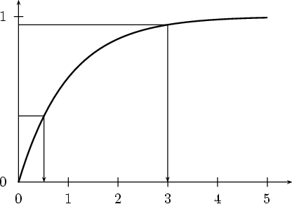
This algorithm is so simple that inversion is certainly the method of choice if the inverse CDF is available in closed form. This is the case e.g. for the exponential and the Cauchy distribution.
The inversion method also has other special advantages that make it even more attractive for simulation purposes. It preserves the structural properties of the underlying uniform pseudo-random number generator. Consequently it can be used, e.g., for variance reduction techniques, it is easy to sample from truncated distributions, from marginal distributions, and from order statistics. Moreover, the quality of the generated random variables depends only on the underlying uniform (pseudo-) random number generator. Another important advantage of the inversion method is that we can easily characterize its performance. To generate one random variate we always need exactly one uniform variate and one evaluation of the inverse CDF. So its speed mainly depends on the costs for evaluating the inverse CDF. Hence inversion is often considered as the method of choice in the simulation literature.
Unfortunately computing the inverse CDF is, for many important standard distributions (e.g. for normal, student, gamma, and beta-distributions), comparatively difficult and slow. Often no such routines are available in standard programming libraries. Then numerical methods for inverting the CDF are necessary, e.g. Newton’s method or (polynomial or rational) approximations of the inverse CDF. Such procedures, however, have the disadvantage that they are not exact and/or slow. UNU.RAN implements several methods: NINV (see NINV – Numerical INVersion), HINV (see HINV – Hermite interpolation based INVersion of CDF) and PINV (see PINV – Polynomial interpolation based INVersion of CDF).
For such approximate inversion methods the approximation error is important for the quality of the generated point set. Let X=G-1(U) denote the approximate inverse CDF, and let F and F-1 be the exact CDF and inverse CDF of the distribution, resp. There are three measures for the approximation error:
- u-error
is given by
uerror = |U-F(G-1(U))|
Goodness-of-fit tests like the Kolmogorov-Smirnov test or the chi-squared test look at this type of error. We are also convinced that it is the most suitable error measure for Monte Carlo simulations as pseudo-random numbers and points of low discrepancy sets are located on a grid of restricted resolution.
- x-error
is given by
absolute xerror = |F-1(U)-G-1(U)|
relative xerror = |F-1(U)-G-1(U)| * |F-1(U)|
The x-error measure the deviation of G-1(U) from the exact result. This measure is suitable when the inverse CDF is used as a quantile function in some computations. The main problem with the x-error is that we have to use the absolute x-error for X=F-1(U) close to zero and the relative x-error in the tails.
We use the terms u-resolution and x-resolution as the maximal tolerated u-error and x-error, resp.
UNU.RAN allows to set u-resolution and x-resolution independently. Both requirements must be fulfilled. We use the following strategy for checking whether the precision goal is reached:
- checking u-error:
The u-error must be slightly smaller than the given u-resolution:
|U-F(G-1(U))| < 0.9 * uresolution.
There is no necessity to consinder the relative u-error as we have 0 < U < 1.
- checking x-error:
We combine absoute and relative x-error and use the criterion
|F-1(U)-G-1(U)| < xresolution * (|G-1(U)| + xresolution).
Remark: It should be noted here that the criterion based on the u-error is too stringent whereever the CDF is extremely steep (and thus the PDF has a pole or a high and narrow peak). This is in particular a problem for distributions with a pole (e.g., the gamma distribution with shape parameter less than 0.5). On the other hand using a criterion based on the x-error causes problems whereever the CDF is extremly flat. This is in particular the case in the (far) tails of heavy-tailed distributions (e.g., for the Cauchy distribution).
Next: The Composition Method, Previous: The Inversion Method, Up: A Short Introduction to Random Variate Generation [Contents][Index]
A.2 The Rejection Method
The rejection method, often called acceptance-rejection method, has been suggested by John von Neumann in 1951. Since then it has proven to be the most flexible and most efficient method to generate variates from continuous distributions.
We explain the rejection principle first for the density f(x) = sin(x)/2 on the interval (0, pi). To generate random variates from this distribution we also can sample random points that are uniformly distributed in the region between the graph of f(x) and the x-axis, i.e., the shaded region in the below figure.
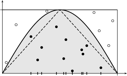
In general this is not a trivial task but in this example we can easily use the rejection trick: Sample a random point (X,Y) uniformly in the bounding rectangle (0, pi)x(0,0.5). This is easy since each coordinate can be sampled independently from the respective uniform distributions U(0, pi) and U(0,0.5). Whenever the point falls into the shaded region below the graph (indicated by dots in the figure), i.e., when Y < sin(X)/2, we accept it and return X as a random variate from the distribution with density f(x). Otherwise we have to reject the point (indicated by small circles in the figure), and try again.
It is quite clear that this idea works for every distribution with a bounded density on a bounded domain. Moreover, we can use this procedure with any multiple of the density, i.e., with any positive bounded function with bounded integral and it is not necessary to know the integral of this function. So we use the term density in the sequel for any positive function with bounded integral.
From the figure we can conclude that the performance of a rejection algorithm depends heavily on the area of the enveloping rectangle. Moreover, the method does not work if the target distribution has infinite tails (or is unbounded). Hence non-rectangular shaped regions for the envelopes are important and we have to solve the problem of sampling points uniformly from such domains. Looking again at the example above we notice that the x-coordinate of the random point (X,Y) was sampled by inversion from the uniform distribution on the domain of the given density. This motivates us to replace the density of the uniform distribution by the (multiple of a) density h(x) of some other appropriate distribution. We only have to take care that it is chosen such that it is always an upper bound, i.e., h(x) >= f(x) for all x in the domain of the distribution. To generate the pair (X,Y) we generate X from the distribution with density proportional to h(x) and Y uniformly between 0 and h(X). The first step (generate X ) is usually done by inversion (see The Inversion Method).
Thus the general rejection algorithm for a hat h(x) with inverse CDF H-1 consists of the following steps:
- Generate a U(0,1) random number U.
- Set X to H-1(U).
- Generate a U(0,1) random number V.
- Set Y to V h(X).
- If Y <= f(X) accept X as the random variate.
- Else try again.
If the evaluation of the density f(x) is expensive (i.e., time consuming) it is possible to use a simple lower bound of the density as so called squeeze function s(x) (the triangular shaped function in the above figure is an example for such a squeeze). We can then accept X when Y <= s(X) and can thus often save the evaluation of the density.
We have seen so far that the rejection principle leads to short and simple generation algorithms. The main practical problem to apply the rejection algorithm is the search for a good fitting hat function and for squeezes. We do not discuss these topics here as they are the heart of the different automatic algorithms implemented in UNU.RAN. Information about the construction of hat and squeeze can therefore be found in the descriptions of the methods.
The performance characteristics of rejection algorithms mainly depend on the fit of the hat and the squeeze. It is not difficult to prove that:
- The expected number of trials to generate one variate is the ratio between the area below the hat and the area below the density.
- The expected number of evaluations of the density necessary to generate one variate is equal to the ratio between the area below the hat and the area below the density, when no squeeze is used. Otherwise, when a squeeze is given it is equal to the ratio between the area between hat and squeeze and the area below the hat.
- The
sqhratio(i.e., the ratio between the area below the squeeze and the area below the hat) used in some of the UNU.RAN methods is easy to compute. It is useful as its reciprocal is an upper bound for the expected number of trials of the rejection algoritm. The expected number of evaluations of the density is bounded by (1/sqhratio)-1.
Next: The Ratio-of-Uniforms Method, Previous: The Rejection Method, Up: A Short Introduction to Random Variate Generation [Contents][Index]
A.3 The Composition Method
The composition method is an important principle to facilitate and speed up random variate generation. The basic idea is simple. To generate random variates with a given density we first split the domain of the density into subintervals. Then we select one of these randomly with probabilities given by the area below the density in the respective subintervals. Finally we generate a random variate from the density of the selected part by inversion and return it as random variate of the full distribution.
Composition can be combined with rejection. Thus it is possible to decompose the domain of the distribution into subintervals and to construct hat and squeeze functions seperatly in every subinterval. The area below the hat must be determined in every subinterval. Then the Composition rejection algorithm contains the following steps:
- Generate the index J of the subinterval as the realisation of a discrete random variate with probabilities proportional to the area below the hat.
- Generate a random variate X proportional to the hat in interval J.
- Generate the U(0,f(X)) random number Y.
- If Y <= f(X) accept X as random variate.
- Else start again with generating the index J.
The first step can be done in constant time (i.e., independent of the number of chosen subintervals) by means of the indexed search method (see Indexed Search (Guide Table Method)).
It is possible to reduce the number of uniform random numbers required in the above algorithm by recycling the random numbers used in Step 1 and additionally by applying the principle of immediate acceptance. For details see [HLD04: Sect. 3.1] .
Next: Inversion for Discrete Distributions, Previous: The Composition Method, Up: A Short Introduction to Random Variate Generation [Contents][Index]
A.4 The Ratio-of-Uniforms Method
The construction of an appropriate hat function for the given density is the crucial step for constructing rejection algorithms. Equivalently we can try to find an appropriate envelope for the region between the graph of the density and the x-axis, such that we can easily sample uniformly distributed random points. This task could become easier if we can find transformations that map the region between the density and the axis into a region of more suitable shape (for example into a bounded region).
As a first example we consider the following simple algorithm for the Cauchy distribution.
- Generate a U(-1,1) random number U and a U(0,1) random number V.
- If U2 + V2 <= 1 accept X=U/V as a Cauchy random variate.
- Else try again.
It is possible to prove that the above algorithm indeed generates Cauchy random variates. The fundamental principle behind this algorithm is the fact that the region below the density is mapped by the transformation
(X,Y) -> (U,V)=(2 Xsqrt(Y),2 sqrt(Y))
into a half-disc in such a way that the ratio between the area of the image to the area of the preimage is constant. This is due to the fact that that the Jacobian of this transformation is constant.
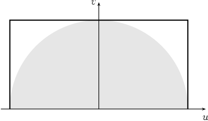
The above example is a special case of a more general principle, called the Ratio-of-uniforms (RoU) method. It is based on the fact that for a random variable X with density f(x) and some constant mu we can generate X from the desired density by calculating X=U/V+ mu for a pair (U,V) uniformly distributed in the set
A_f= { (u,v) : 0 < v <= sqrt(f(u/v+ mu)) } .
For most distributions it is best to set the constant mu equal to the mode of the distribution. For sampling random points uniformly distributed in A_f rejection from a convenient enveloping region is used, usually the minimal bounding rectangle, i.e., the smallest possible rectangle that contains A_f (see the above figure). It is given by (u-,u+)x(0,v+) where
v+ = sup_b_l<x<b_r sqrt(f(x)),
u- = inf_b_l<x<b_r (x- mu) sqrt(f(x)),
u+ = sup_b_l<x<b_r (x- mu) sqrt(f(x)).
Then the ratio-of-uniforms method consists of the following simple steps:
- Generate a U(u-,u+) random number U and a U(0,v+) random number V.
- Set X to U/V+ mu.
- If V2 <= f(X) accept X as the random variate.
- Else try again.
To apply the ratio-of-uniforms algorithm to a certain density we have to solve the simple optimization problems in the definitions above to obtain the design constants u-, u+, and v+. This simple algorithm works for all distributions with bounded densities that have subquadratic tails (i.e., tails like 1/x2 or lower). For most standard distributions it has quite good rejection constants. (E.g. 1.3688 for the normal and 1.4715 for the exponential distribution.)
Nevertheless, we use more sophisticated method that construct better fitting envelopes, like method AROU (see AROU – Automatic Ratio-Of-Uniforms method), or even avoid the computation of these design constants and thus have almost no setup, like method SROU (see SROU – Simple Ratio-Of-Uniforms method).
The Generalized Ratio-of-Uniforms Method
The Ratio-of-Uniforms method can be generalized: If a point (U,V) is uniformly distributed in the set
A_f= { (u,v) : 0 < v <= (f(u/vr+ mu))1/(r+1) }
then X=U/Vr+ mu has the denity f(x). The minimal bounding rectangle of this region is given by (u-,u+)x(0,v+) where
v+ = sup_b_l<x<b_r (f(x))1/(r+1),
u- = inf_b_l<x<b_r (x- mu) (f(x))r/(r+1),
u+ = sup_b_l<x<b_r (x- mu) (f(x))r/(r+1).
The above algorithm has then to be adjusted accordingly. Notice that the original Ratio-of-Uniforms method is the special case with r=1.
Next: Indexed Search (Guide Table Method), Previous: The Ratio-of-Uniforms Method, Up: A Short Introduction to Random Variate Generation [Contents][Index]
A.5 Inversion for Discrete Distributions
We have already presented the idea of the inversion method to generate from continuous random variables (see The Inversion Method). For a discrete random variable X we can write it mathematically in the same way:
X=F-1(U),
where F is the CDF of the desired distribution and U is a uniform U(0,1) random number. The difference compared to the continuous case is that F is now a step-function. The following figure illustrates the idea of discrete inversion for a simple distribution.
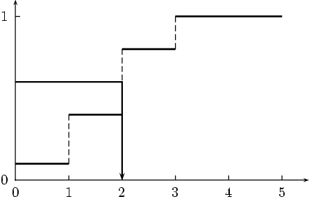
To realize this idea on a computer we have to use a search algorithm. For the simplest version called Sequential Search the CDF is computed on-the-fly as sum of the probabilities p(k), since this is usually much cheaper than computing the CDF directly. It is obvious that the basic form of the search algorithm only works for discrete random variables with probability mass functions p(k) for nonnegative k. The sequential search algorithm consists of the following basic steps:
- Generate a U(0,1) random number U.
- Set X to 0 and P to p(0).
- Do while U > P
- Set X to X+1 and P to P+p(X).
- Return X.
With the exception of some very simple discrete distributions, sequential search algorithms become very slow as the while-loop has to be repeated very often. The expected number of iterations, i.e., the number of comparisons in the while condition, is equal to the expectation of the distribution plus 1. It can therefore become arbitrary large or even infinity if the tail of the distribution is very heavy. Another serious problem can be critical round-off errors due to summing up many probabilities p(k). To speed up the search procedure it is best to use indexed search.
Previous: Inversion for Discrete Distributions, Up: A Short Introduction to Random Variate Generation [Contents][Index]
A.6 Indexed Search (Guide Table Method)
The idea to speed up the sequential search algorithm is easy to understand. Instead of starting always at 0 we store a table of size C with starting points for our search. For this table we compute F-1(U) for C equidistributed values of U, i.e., for u_i = i/C, i=0,...,C-1. Such a table is called guide table or hash table. Then it is easy to prove that for every U in (0,1) the guide table entry for k=floor(UC) is bounded by F-1(U). This shows that we can really start our sequential search procedure from the table entry for k and the index k of the correct table entry can be found rapidly by means of the truncation operation.
The two main differences between indexed search and sequential search are that we start searching at the number determined by the guide table, and that we have to compute and store the cumulative probabilities in the setup as we have to know the cumulative probability for the starting point of the search algorithm. The rounding problems that can occur in the sequential search algorithm can occur here as well. Compared to sequential search we have now the obvious drawback of a slow setup. The computation of the cumulative probabilities grows linear with the size of the domain of the distribution L. What we gain is really high speed as the marginal execution time of the sampling algorithm becomes very small. The expected number of comparisons is bounded by 1+L/C. This shows that there is a trade-off between speed and the size of the guide table. Cache-effects in modern computers will however slow down the speed-up for really large table sizes. Thus we recommend to use a guide table that is about two times larger than the probability vector to obtain optimal speed.
Next: Bibliography, Previous: A Short Introduction to Random Variate Generation, Up: UNU.RAN – Universal Non-Uniform RANdom number generators [Contents][Index]
Appendix B Glossary
- CDF
cumulative distribution function.
- HR
hazard rate (or failure rate).
- inverse local concavity
local concavity of inverse PDF f-1(y) expressed in term of x = f-1(y). Is is given by ilc_f(x) = 1 + x f''(x) / f'(x)
- local concavity
maximum value of c such that PDF f(x) is T_c. Is is given by lc_f(x) = 1 - f''(x) f(x) / f'(x)2
probability density function.
- dPDF
derivative (gradient) of probability density function.
- PMF
probability mass function.
- PV
(finite) probability vector.
- URNG
uniform random number generator.
- U(a,b)
continuous uniform distribution on the interval (a,b).
- T-concave
a function f(x) is called T-convace if the transformed function T(f(x)) is concave. We only deal with transformations T_c, where
c = 0- T(x) = log(x)
c = -0.5- T(x) = -1/sqrt(x)
c != 0- T(x) = sign(x) * xc
- u-error
for a given approximate inverse CDF X=G-1(U) the u-error is given as
uerror = |U-F(G-1(U))|
where F denotes the exact CDF. Goodness-of-fit tests like the Kolmogorov-Smirnov test or the chi-squared test look at this type of error. See The Inversion Method for more details.
- u-resolution
the maximal tolerated u-error for an approximate inverse CDF.
- x-error
for a given approximate inverse CDF X=G-1(U) the x-error is given as
xerror = |F-1(U)-G-1(U)|
where F-1 denotes the exact inverse CDF. The x-error measure the deviation of G-1(U) from the exact result. Notice that we have to distinguish between absolute and relative x-error. In UNU.RAN we use the absolute x-error near 0 and the relative x-error otherwise. See The Inversion Method for more details.
- x-resolution
the maximal tolerated x-error for an approximate inverse CDF.
Next: Function Index, Previous: Glossary, Up: UNU.RAN – Universal Non-Uniform RANdom number generators [Contents][Index]
Appendix C Bibliography
Standard Distributions
[JKKa92]N.L. JOHNSON, S. KOTZ, AND A.W. KEMP (1992). Univariate Discrete Distributions, 2nd edition, John Wiley & Sons, Inc., New York.
[JKBb94]N.L. JOHNSON, S. KOTZ, AND N. BALAKRISHNAN (1994). Continuous Univariate Distributions, Volume 1, 2nd edition, John Wiley & Sons, Inc., New York.
[JKBc95]N.L. JOHNSON, S. KOTZ, AND N. BALAKRISHNAN (1995). Continuous Univariate Distributions, Volume 2, 2nd edition, John Wiley & Sons, Inc., New York.
[JKBd97]N.L. JOHNSON, S. KOTZ, AND N. BALAKRISHNAN (1997). Discrete Multivariate Distributions, John Wiley & Sons, Inc., New York.
[KBJe00]S. KOTZ, N. BALAKRISHNAN, AND N.L. JOHNSON (2000). Continuous Multivariate Distributions, Volume 1: Models and Applications, John Wiley & Sons, Inc., New York.
Universal Methods – Surveys
[HLD04]W. HÖRMANN, J. LEYDOLD, AND G. DERFLINGER (2004). Automatic Nonuniform Random Variate Generation, Springer, Berlin.
Universal Methods
[AJa93]J.H. AHRENS (1993). Sampling from general distributions by suboptimal division of domains, Grazer Math. Berichte 319, 30pp.
[AJa95]J.H. AHRENS (1995). An one-table method for sampling from continuous and discrete distributions, Computing 54(2), pp. 127-146.
[CAa74]H.C. CHEN AND Y. ASAU (1974). On generating random variates from an empirical distribution, AIIE Trans. 6, pp. 163-166.
[DHLa08]G. DERFLINGER, W. HÖRMANN, AND J. LEYDOLD (2008). Numerical inversion when only the density function is known, Research Report Series of the Department of Statistics and Mathematics 78, WU Wien, Augasse 2–6, A-1090 Wien, Austria, http://epub.wu.ac.at/english/.
[DLa86]L. DEVROYE (1986). Non-Uniform Random Variate Generation, Springer Verlag, New York.
[GWa92]W.R. GILKS AND P. WILD (1992). Adaptive rejection sampling for Gibbs sampling, Applied Statistics 41, pp. 337-348.
[HWa95]W. HÖRMANN (1995). A rejection technique for sampling from T-concave distributions, ACM Trans. Math. Software 21(2), pp. 182-193.
[HDa96]W. HÖRMANN AND G. DERFLINGER (1996). Rejection-inversion to generate variates from monotone discrete distributions, ACM TOMACS 6(3), 169-184.
[HLa00]W. HÖRMANN AND J. LEYDOLD (2000). Automatic random variate generation for simulation input. In: J.A. Joines, R. Barton, P. Fishwick, K. Kang (eds.), Proceedings of the 2000 Winter Simulation Conference, pp. 675-682.
[HLa03]W. HÖRMANN AND J. LEYDOLD (2003). Continuous Random Variate Generation by Fast Numerical Inversion, ACM TOMACS 13(4), 347-362.
[HLDa07]W. HÖRMANN, J. LEYDOLD, AND G. DERFLINGER (2007). Automatic Random Variate Generation for Unbounded Densities, ACM Trans. Model. Comput. Simul. 17(4), pp.18.
[KLPa05]R. KARAWATZKI, J. LEYDOLD, AND K. PÖTZELBERGER (2005). Automatic Markov chain Monte Carlo procedures for sampling from multivariate distributions, Research Report Series of the Department of Statistics and Mathematics 27, WU Wien, Augasse 2–6, A-1090 Wien, Austria, http://epub.wu.ac.at/english/.
[LJa98]J. LEYDOLD (1998). A Rejection Technique for Sampling from Log-Concave Multivariate Distributions, ACM TOMACS 8(3), pp. 254-280.
[LJa00]J. LEYDOLD (2000). Automatic Sampling with the Ratio-of-Uniforms Method, ACM Trans. Math. Software 26(1), pp. 78-98.
[LJa01]J. LEYDOLD (2001). A simple universal generator for continuous and discrete univariate T-concave distributions, ACM Trans. Math. Software 27(1), pp. 66-82.
[LJa02]J. LEYDOLD (2003). Short universal generators via generalized ratio-of-uniforms method, Math. Comp. 72(243), pp. 1453-1471.
[WGS91]J.C. WAKEFIELD, A.E. GELFAND, AND A.F.M. SMITH (1992). Efficient generation of random variates via the ratio-of-uniforms method, Statist. Comput. 1(2), pp. 129-133.
[WAa77]A.J. WALKER (1977). An efficient method for generating discrete random variables with general distributions, ACM Trans. Math. Software 3, pp. 253-256.
Special Generators
[ADa74]J.H. AHRENS, U. DIETER (1974). Computer methods for sampling from gamma, beta, Poisson and binomial distributions, Computing 12, 223-246.
[ADa82]J.H. AHRENS, U. DIETER (1982). Generating gamma variates by a modified rejection technique, Communications of the ACM 25, 47-54.
[ADb82]J.H. AHRENS, U. DIETER (1982). Computer generation of Poisson deviates from modified normal distributions, ACM Trans. Math. Software 8, 163-179.
[BMa58]G.E.P. BOX AND M.E. MULLER (1958). A note on the generation of random normal deviates, Annals Math. Statist. 29, 610-611.
[CHa77]R.C.H. CHENG (1977). The Generation of Gamma Variables with Non-Integral Shape Parameter, Appl. Statist. 26(1), 71-75.
[Dag89]J.S. DAGPUNAR (1989). An Easily Implemented Generalised Inverse Gaussian Generator, Commun. Statist. Simul. 18(2), 703-710.
[HDa90]W. HÖRMANN AND G. DERFLINGER (1990). The ACR Method for generating normal random variables, OR Spektrum 12, 181-185.
[KAa81]A.W. KEMP (1981). Efficient generation of logarithmically distributed pseudo-random variables, Appl. Statist. 30, 249-253.
[KRa76]A.J. KINDERMAN AND J.G. RAMAGE (1976). Computer Generation of Normal Random Variables, J. Am. Stat. Assoc. 71(356), 893 - 898.
[MJa87]J.F. MONAHAN (1987). An algorithm for generating chi random variables, ACM Trans. Math. Software 13, 168-172.
[MGa62]G. MARSAGLIA (1962). Improving the Polar Method for Generating a Pair of Random Variables, Boeing Sci. Res. Lab., Seattle, Washington.
[MOa84]G. MARSAGLIA AND I. OLKIN (1984). Generating Correlation Matrices, SIAM J. Sci. Stat. Comput 5, 470-475.
[STa89]E. STADLOBER (1989). Sampling from Poisson, binomial and hypergeometric distributions: ratio of uniforms as a simple and fast alternative, Bericht 303, Math. Stat. Sektion, Forschungsgesellschaft Joanneum, Graz.
[ZHa94]H. ZECHNER (1994). Efficient sampling from continuous and discrete unimodal distributions, Pd.D. Thesis, 156 pp., Technical University Graz, Austria.
Other references
[CPa76]R. CRANLEY AND T.N.L. PATTERSON (1976). Randomization of number theoretic methods for multiple integration, SIAM J. Num. Anal., Vol. 13, pp. 904-914.
[HJa61]R. HOOKE AND T.A. JEEVES (1961). Direct Search Solution of Numerical and Statistical Problems, Journal of the ACM, Vol. 8, April 1961, pp. 212-229.
Previous: Bibliography, Up: UNU.RAN – Universal Non-Uniform RANdom number generators [Contents][Index]