Star Map 2D

Star Map 2D // A self-organizing map of the 5000 closest stars

Our sci-fi books, movies and games are filled with exploration of the galaxy and the universe at large. It’s all planet this and star system that, and how many parsecs between them.

But notice one thing: those places are either completely made up¹ or they are random stars taken from our night sky without any context.²

The reason is that most people (including writers, screenwriters and game masters) don’t actually have any idea what the topology of our star neighbourhood is like. The three dimensions are super confusing. Is Sirius close to Mirzam? They are on the night sky (Mirzam is a bright star right next to Sirius) but they are most definitely not in 3D space (Sirius is 9 light years away, Mirzam is 500).³

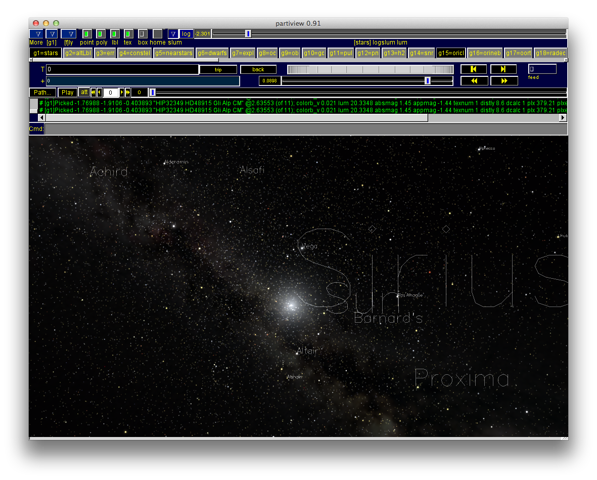
Even if you have a 3D atlas of stars which allows you to travel freely through virtual space, like Digital Universe or Redshift, that experience is no less confusing. Humans are not good at navigating through true three-dimensional space.⁴ Even simple things like trying to find clusters of stars are extremely difficult.

Compare this to a traditional (2D) map. It’s very easy for us humans to see that two cities are close to each other, for example. At a glance, we can see clusters, gaps, strings, and so on. We can plan and reason about the map.

The problem of 2D star maps

There are 2D star maps already, of course – Winchell D. Chung’s maps being probably the best examples. So why make another?

The problem is that the currently available 2D maps are views. They show each star at its proper X and Y coordinates, but they completely discard the Z (depth) coordinate. In this respect they are almost as bad a representation of reality as the night sky. Two adjancent stars are often actually quite far from each other – but the viewer doesn’t know this until after they have read that information.⁵

So again, similarly to 3D virtual atlases, with 2D views it’s not easy to do basic things at a glance.

The perfect map

It’s obvious that any 2D map of 3D space will be imperfect. But we can still do better than a view. Let these be our goals for the map:

• Instances of outright lies (for example, Sirius and Mirzam rendered next to each other) are minimized.
• It is possible to make basic observations about the depicted stars at a glance, with a reasonable level of certainty. For example:
  • Identify clusters of stars.
  • See if star is solitary (no close neighbours).
  • See what stars are neighbouring any given star.
• If star C is three times farther away from star B than star A in space, we want to see the same thing on the map.⁶

Note also what isn’t our goal here: perfect representation of 3D space on a 2D map. We are trying to minimize the distortion but we can’t ever hope to get rid of it completely.

Enter Teuvo Kohonen

But even when we limit our goals and recognize that the map can’t be perfect, it’s very hard to create a suitable map for even a few stars, and virtually impossible to do so for thousands of them…

… UNLESS YOU HAVE THINKING MACHINES THAT CAN DO THE WORK FOR YOU.

Which we have. Thanks to the amazing thing that is general purpose computing, and thanks to a particularly clever algorithm by the Finnish academician Teuvo Kohonen, we can leave the work to the machines.

A self-organizing map is an artificial neural network that learns to represent multi-dimensional data on a (usually 2D) map. It can be used to analyze huge data tables – for example, a university’s students can be plotted on a self-organizing map according to their grades in different courses. Such a map can then help in finding students with similar strengths and weaknesses.

Turns out a star’s 3D coordinates can be seen as multi-dimensional data. Because that’s exactly what they are. :)

I simply applied a well-documented algorithm to an obvious-in-retrospect dataset.

Of course, it wasn’t that simple to actually arrive at something usable. It took me 5 months to find the winning formula⁷ – there are many parameters that have to be chosen by experimentation, and every training of such a large Kohonen network takes anything from half a day to more than a month of continuous CPU usage.

Specifications

• The map consists of 848x600 hexagonal tiles.
  • The aspect ratio is √2:1,⁸ same as the international paper size A standard (A4, A3, A2, etc.).
• The map is toroidal (‘wrap around’).
  • In other words, opposite edges of the map are connected. This means that, for example, ‘going through’ the top edge ‘teleports’ you to the bottom. If you remember the game Asteroids, you probably know what I mean.
  • The reason for this is because it is easier for the 2D self-organizing map to be weaved through the 3D space if it’s toroidal, which means less distortion.
• There are exactly 5000 stars on the map.
  • They are Sol (the Sun) and the 4999 known stars closest to it from David Nash’s HYG Database.
  • It’s a sphere of stars 72 light years in diameter, with Sol at its center.
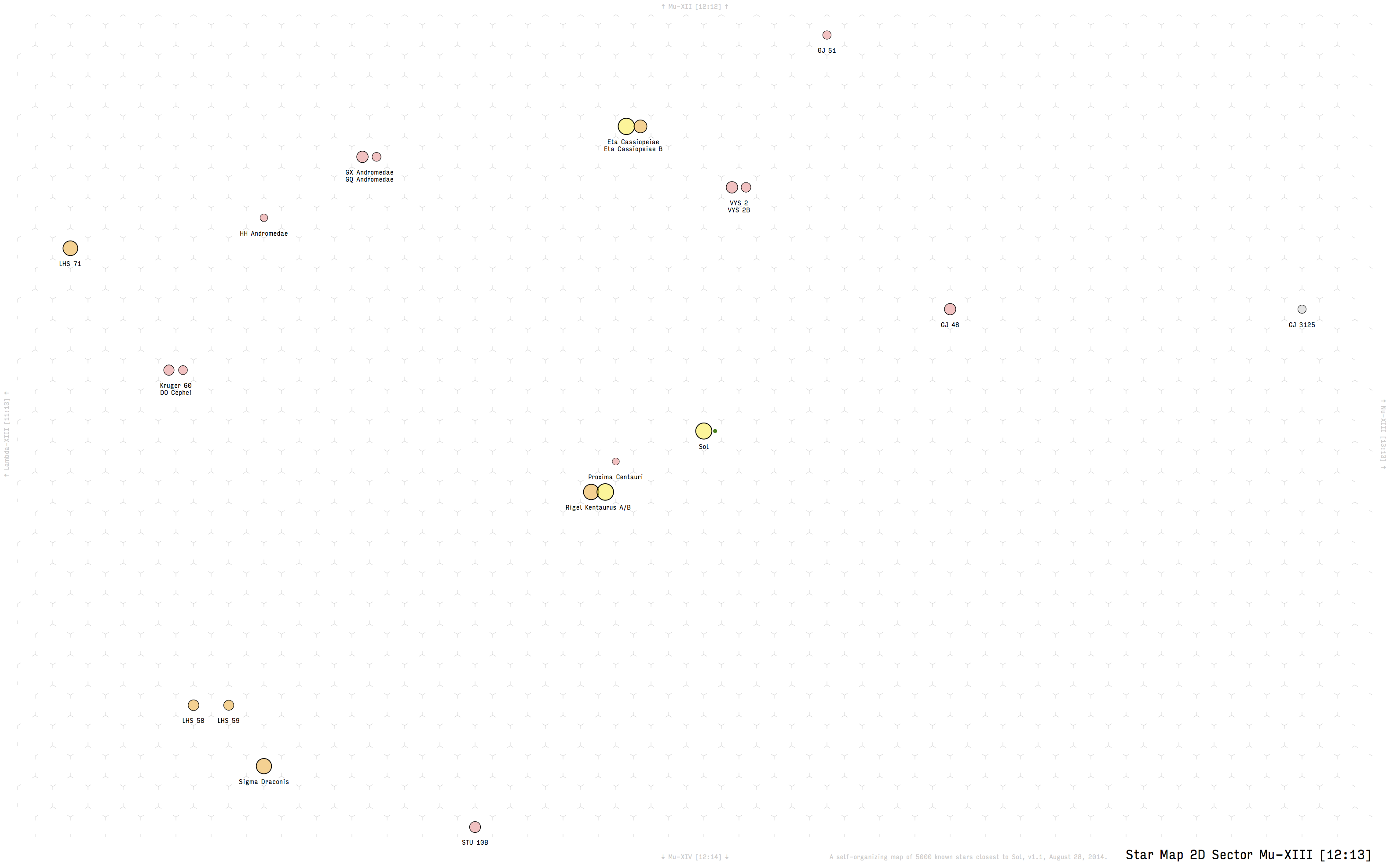
• Legend:
  • Stars are color-coded by spectral type.
  • The size of a star on the map corresponds to its absolute magnitude – larger is brighter.
  • Stars with a little green dot next to them are candidates to have a habitable, Earth-like planet on their orbit.⁹
• One hex on the map is approximately 1 light year in space.¹⁰

Gallery

Download

Both bundles below include an overview map (PDF), a meta-map of sectors NOT AVAILABLE YET, all the 576 sectors (PDFs), index files, and the CSV file with all the raw data.

• ‘Scientific’ bundle NOT AVAILABLE YET
  • Stars are mostly labeled by their standard catalogue codes (for example: HIP 89937). This makes it very easy to research each star on astrological databases such as Simbad. This also makes the map pretty boring.
• ‘Literary’ bundle (v1.4, ~29MB, zip)
  • Stars are either labeled by a proper name (for example: Aldebaran) or by a constellation-based name (for example: Chi Draconis). If none of those two is available, a cool-sounding catalogue code¹¹ is chosen over a more commonly used one (for example: STU 10B is chosen over HIP 86162).
• Standalone files:
  • CSV file (v1.4, ~500kB)
    • One row per star, with a ‘literary’ name, a ‘scientific’ code, 2D coordinates, 3D coordinates, habitability, and other datapoints for each.

The PDF files do not contain the font (Input Sans Condensed) that you see in the screenshots above. You can download the font here (free for personal use).

What to do with this?

Wouldn’t it be nice to see a fictional empire, federation, space-faring nation or civilization that inhabits stars that are actually close to each other? If you’re writing a book, screenwriting, creating a game or running a role-playing adventure set in space, consider using the map. (I’d be thrilled if you tell me.)

This was, by the way, my original motivation for creating the 2D Star Map in the first place. I am using this for my gamebook / free exploration game called The Bodega Incident. You can learn more about that project at egamebook.com.

If you’re a (hobby) astronomer, you might like the idea of seeing stars in their context without having to fire up 3D software every time.

Suggested use:

1. Pick a star and find out which sector it is in.
   • Or, just pick a sector randomly.
2. Print out the sector and it’s neighbours.
   • Based on the epicness of your project, you can print out just 1, or four, or 16 papers, or whatever.
3. Arrange them on the floor or on the table.
   • The little notes on the sides are a hint for you about what comes where.
   • Keep in mind that each page has a 1-hex border at each side that belongs to the neighbouring sector.
4. Start planning your galactic conquest (or whatever else it is you’re doing).

Index of well-known stars

Star name	X, Y	Sector
Aldebaran	563, 144	Pi-VI [16:6]
Alderamin	379, 559	Lambda-XXIII [11:23]
Algol	485, 84	Xi-IV [14:4]
Alhena	615, 96	Sigma-IV [18:4]
Alioth	473, 480	Xi-XX [14:20]
Alkaid	450, 468	Nu-XIX [13:19]
Alnair	120, 217	Delta-IX [4:9]
Alphekka	351, 439	Kappa-XVIII [10:18]
Alpheratz	340, 85	Kappa-IV [10:4]
Altair	348, 317	Kappa-XIII [10:13]
Ankaa	105, 149	Gamma-VI [3:6]
Arcturus	424, 382	Mu-XVI [12:16]
Barnard’s Star	393, 318	Lambda-XIII [11:13]
Capella	521, 25	Omicron-II [15:2]
Caph	411, 11	Mu-I [12:1]
Castor	632, 9	Sigma-I [18:1]
Denebola	511, 368	Omicron-XV [15:15]
Diphda	166, 139	Epsilon-VI [5:6]
Fomalhaut	109, 21	Delta-I [4:1]
Groombridge 1618	458, 326	Nu-XIV [13:14]
Groombridge 1830	478, 358	Xi-XV [14:15]
Hamal	427, 127	Mu-VI [12:6]
Kapteyn’s Star	784, 32	Chi-II [22:2]
Kruger 60	399, 310	Mu-XIII [12:13]
Lacaille 8760	89, 597	Gamma-XXIV [3:24]
Lacaille 9352	378, 300	Lambda-XIII [11:13]
Lalande 21185	439, 321	Nu-XIII [13:13]
Luyten’s Star	471, 308	Xi-XIII [14:13]
Merak	519, 501	Omicron-XXI [15:21]
Mizar	458, 474	Nu-XIX [13:19]
Phad	507, 485	Omicron-XX [15:20]
Pollux	528, 312	Omicron-XIII [15:13]
Procyon	467, 310	Nu-XIII [13:13]
Proxima Centauri	411, 313	Mu-XIII [12:13]
Rasalhague	284, 389	Theta-XVI [8:16]
Regulus	640, 451	Sigma-XIX [18:19]
Rigel Kentaurus A	411, 314	Mu-XIII [12:13]
Rigel Kentaurus B	411, 314	Mu-XIII [12:13]
Sirius	447, 306	Nu-XIII [13:13]
Sol	414, 312	Mu-XIII [12:13]
Unukalhai	138, 472	Delta-XIX [4:19]
Van Maanen’s Star	393, 290	Lambda-XII [11:12]
Vega	356, 339	Kappa-XIV [10:14]
Vindemiatrix	756, 483	Chi-XX [22:20]
p Eridani	14, 39	Alpha-II [1:2]

Stars that are well known but are outside the scope of the map:¹² Achernar (44), Acrux (98), Adhara (132), Alcyone (112), Algenib (102), Algieba (38), Alnath (40), Alnilam (411), Alnitak (250), Alphard (54), Antares (185), Arneb (393), Bellatrix (74), Betelgeuse (131), Canopus (95), Deneb (990), Dubhe (37), Enif (206), Etamin (45), Hadar (161), Izar (64), Kaus Australis (44), Kochab (38), Markab (42), Menkar (67), Mirach (61), Mirphak (181), Nihal (48), Nunki (68), Polaris (132), Rasalgethi (117), Rigel (236), Saiph (221), Scheat (61), Shaula (215), Shedir (70), Spica (80), Tarazed (141).

CC License

The underlying data is public domain, of course. I am releasing the computed 2D coordinates to public domain, too. Everything else (the hex maps, the indexes, this text) are CC-BY 4.0.

I am Filip H. and you can reach me at filip dot hracek at gmail dot com or on Twitter.