Arda Goreci · May 20, 2026
Over the last few years, deep neural networks have made generative language modeling dramatically more powerful, giving us large language models. A similar leap happened for continuous modalities like images and videos. Recently, similar techniques have been applied to the generative modeling of biomolecules with great success. Models such as DeepMind's AlphaFold3 made it much easier to predict biomolecular interactions, including drug-protein and antibody-protein complexes, and soon after people figured out how to re-purpose these capabilities to design drug-like molecules. Chai-2, Latent-X2, and Nabla all report developable antibody or biologics designs. In the near future, we might see most antibodies entering the clinic designed in large part with deep-learning-based generative models, potentially with superior pharmaceutical properties and targeting receptors that have resisted wet-lab based approaches.
How would you improve on these systems? We definitely want to have better biomolecular modeling so we can put better drugs into the clinic. The recipe for improving a deep learning system has been surprisingly simple at a high level: you scale the model, scale the compute, and scale the data. LLMs are obviously improving by being scaled aggressively. AlphaFold3 was also a major effort to scale the model and data; it is trained on a broad collection of known biomolecular complexes, from experimental structures and protein-ligand complexes to the enormous sequence databases produced by genomics and metagenomics such as MGnify. Internally, DeepMind called the project "all-PDB" for a while, referring to all the interactions represented in the Protein Data Bank.
The key move in AlphaFold3's scaling recipe was to turn sequence scale into structure scale: use structure prediction to convert large protein sequence databases into predicted 3D structures. Genomics and metagenomics have given us billions of protein sequences, many inferred from environmental DNA collected from organisms that have never been cultured in the lab. For training structure-based design models, though, the useful object is often the 3D structure. Structure prediction models let us convert some of that sequence scale into structural data: take millions of natural sequences, predict the folds they adopt, and use those predicted structures as training examples for the next generation of biomolecular models.
At Ligo, we care about this recipe because we train generative models for designing enzymes. When we tried to scale our structural training data by folding more natural sequences, we ran into a problem: natural protein sequences are vast, but their folds are much more redundant than the sequence counts suggest. This post is about that mismatch, and about why simply folding more natural sequences may not buy as much new structural diversity as we hoped. We will describe data engineering tricks for clustering the known protein universe, and what our results imply about how to think about the enzyme design problem.
Modern biomolecular models rely on sequence scale
Modern structure prediction models rely heavily on multiple sequence alignments. A multiple sequence alignment, or MSA, lines up related versions of a protein from different organisms. When two positions in that alignment tend to change together, Coevolution means that two positions change in a coordinated way across related proteins. For example, if one position is usually negatively charged and touches a positively charged position, evolution may flip both together while avoiding pairs that would repel each other. it can be a clue that the corresponding residues are close in 3D space or tied together by function. My mental model of AlphaFold2 is that it used this kind of coevolutionary signal to constrain the rough geometry of a protein, then learned how to fill in the rest of the structure.
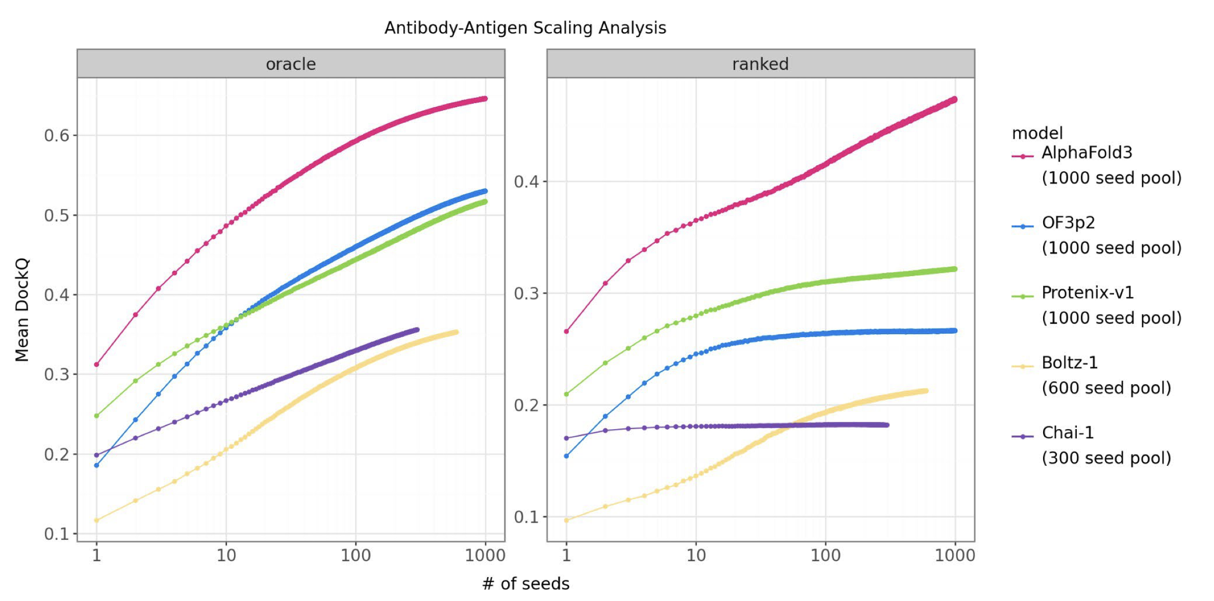
AlphaFold3 seems to be doing something broader. Its antibody-antigen performance is especially interesting because there are no MSAs to extract clues from. Antibodies and their targets do not share an evolutionary history. To do well there, the model has to learn something about protein surfaces themselves: which shapes, chemistries, and local geometries are likely to be compatible with each other. That is a different kind of signal than residue coevolution within one protein family.
This is where MGnify-scale data may matter. Metagenomic sequence resources expose models to enormous numbers of natural variants, many from organisms we have never cultured. The empirical clue is that models trained with MGnify-scale protein distillation seem to separate most clearly on antibody-antigen prediction, where direct coevolution cannot explain the interaction signal (Supplementary info). That increased coverage of sequence space looks valuable. The question is whether it also comes with comparable diversity in protein folds.
Sequence diversity is not fold diversity
The theoretical protein sequence space is absurdly large: a protein of length N has 20N possible amino-acid sequences. Natural proteins occupy only a tiny, highly structured part of that space. Evolution tends to reuse folds that are stable, expressible, and adaptable, rather than scattering proteins uniformly across every possible sequence and shape.
That matters for training data. When we scale predicted structures, we are not necessarily adding independent examples. We may also be adding many sequence variants of the same fold families, domain combinations, and evolutionary compromises. The example below shows the basic problem: proteins can look far apart when measured by sequence similarity, while still being very close in fold space.
One concrete example from our AFDB fragment clusters: in structural cluster
A0A242HMU2_f1, three proteins are only 23.9–28.3% identical in sequence
while still sharing the same fold (TM-score > 0.75).
Pairwise global identities after clipping: 28.2%, 28.3%, and 23.9%.
Local TM-align scores on the predicted structures are 0.768–0.813
using average-length normalization.
| Fragment | UniProt annotation | Length | Seq. id. to rep. | TM to rep. |
|---|---|---|---|---|
A0A518BRX6_f1 |
3-oxoacyl-[acyl-carrier-protein] reductase FabG, Bacteria | 249 aa | 100% | 1.000 |
A0A1Q3EPK1_f1 |
NAD-binding protein, Lentinula edodes | 283 aa | 28.2% | 0.768 |
A0A6I8MDZ6_f1 |
Short-chain dehydrogenase/reductase SDR, Oceanivirga miroungae | 261 aa | 23.9% | 0.793 |
Same fold, low sequence identity
Three AFDB predictions from the same structural cluster, aligned with local TM-align.
A FabG reductase
B SDR protein
C clipped NAD-binding core
Loading aligned fold overlay...
As we scale up our sequence datasets, how many genuinely new folds should we expect to see? If MGnify grew 10x, how many of those new sequences would actually be structurally novel?
To answer this systematically across the whole space, we need a scalable clustering algorithm. Foldseek is a brilliant tool for this, and its authors have already clustered the AlphaFold Database with it, reporting 2.3 million non-singleton structural clusters. But there are real issues with clustering predicted structures, and the clustering problem itself is ill-posed. We think the true number of reusable structural neighborhoods is much closer to tens of thousands than to the 2.3 million non-singleton clusters reported by that fast Foldseek pass — closer to 25,000 than 2.3 million in our current analysis. Here's the reasoning.
The predicted-structure problem for clustering
Predicted structures are different from crystals. The sequences and MSAs are real, but the structures are missing context, and AlphaFold will predict the whole chain: ordered domains, floppy tails, long linkers, signal peptides, and multi-domain proteins whose relative placement may not be meaningful.
This makes the clustering problem ill-posed. Are two proteins the same fold because one domain matches? Are they different because one has a disordered extension?
The shape of predicted structures is also a problem for training generative models on this data. You don't want to waste model capacity fitting disordered regions, and you don't want to learn to generate bizarre, elongated chains. You could filter on global pLDDT, radius of gyration, and similar whole-chain metrics, but those filters are too crude for data shaped like this — they throw out good domains attached to bad tails. We need a more surgical way to keep the signal and drop the noise.
Predicted chains are not clean domains
very high confident low very low
A0A5B2Z7Q7, ArsR-family transcriptional regulator
Waiting to load...
P38398-3, breast cancer type 1 susceptibility protein isoform (BRCA1)
Waiting to load...
First pass: remove the obvious noise
Our first attempt was simple. Remove residues below a pLDDT threshold, split what remains into contiguous sequence fragments, and then spatially rejoin fragments that are clearly touching. The rejoin step is a union-find problem: if fragment A touches B, and B touches C, then A, B, and C become one connected fragment.
- Residues below pLDDT 65 are marked as unusable.
- Remaining residues become contiguous sequence fragments.
- Fragments with enough close contacts are merged spatially.
- The resulting candidates can then be filtered before clustering.
This gets rid of a lot of obvious disorder. It also keeps ordered domains that global filters would throw away because the full protein looked too long, too extended, or too messy.
Limitations of naive fragmentation. The obvious failure mode is a high-confidence linker. If the linker survives the pLDDT filter and makes enough contacts, the spatial merge can connect two domains that we would rather treat separately. Union-find then does exactly what it was asked to do: it turns the connected chain into one fragment.
The problem is that this is not really a local-confidence question. The residues can be predicted confidently and still be the wrong unit of training. What we need to detect is the bottleneck in the spatial graph: the narrow path that connects otherwise independent pieces.
A0A0E0RCK4 first pass
The full chain is kept intact; fragments shorter than 20 residues are left unnumbered.
Waiting to load...
The graph-theoretic split
We need a way to split proteins based on how the residues are connected to each other. For that, a protein is naturally a graph: each residue is a node, and edges connect residues that are close in space. We use C-alpha atoms from the confident part of the prediction, connect each residue to its spatial nearest neighbors, and give close neighbors stronger weights than distant ones. In the current version, each residue sees its 15 nearest spatial neighbors.
This turns the fragmentation problem into a connectivity problem. A compact domain becomes a dense local graph. A high-confidence linker becomes a narrow bridge between two dense regions. Graph theory gives us tools for asking whether that bridge is really part of one unit, or whether it is holding two independent pieces together.
Graph theoretic split of a nearest neighbour protein graph
Waiting to load...
Fiedler vector
Spectral bisection asks for the weakest global connection in this graph (why the quantity we compute finds this connection is a little bit black magic to me, ask the graph theorists). We found that the spectral bisection points of a protein correlate very well with the points we'd cut at if we were manually identifying different protein regions. A standalone version of the splitter is included in Supplementary info.
For the curious: the Fiedler vector
Given a weighted adjacency matrix \(W\) of a graph, the normalized graph Laplacian is:
\[ L_{\mathrm{sym}} = I - D^{-1/2} W D^{-1/2} \]
Here \(D\) is the diagonal degree matrix. The eigenvectors of \(L_{\mathrm{sym}}\) reveal graph structure:
- The smallest eigenvalue is always 0.
- The second smallest eigenvalue, \(\lambda_2\), measures algebraic connectivity.
- The corresponding Fiedler vector gives a useful two-way partition: residues with opposite signs sit on opposite sides of the cut.
This is the same quantity shown on the graph above. The protein is just green context, while the graph edges are colored by the average Fiedler value of their two endpoint residues. Strongly negative edges are blue, strongly positive edges are red, and edges near zero are pale. Those near-zero residues are the bottleneck between the two sides, so those are the residues we remove before assigning fragments.
Recursive bisection
A single bisection only finds one cut. Multi-domain proteins need repeated
cuts, so after each split we check each partition separately. If a
partition has λ2 > threshold, we treat it
as internally well connected and stop. Otherwise, we split again.
Naive merge versus spectral pipeline
Both panels load one full-chain CIF; fragments shorter than 20 residues are left unnumbered.
Waiting to load...
Waiting to load...
Clustering the fragments
Once we split proteins into their "interacting units", the unit of clustering is no longer one predicted protein. It is one compact fragment. We can cluster those fragments by structural similarity and ask how much independent fold signal the distillation sets actually contain.
We cluster MGnify at roughly 30% sequence identity with MMseqs2, which gives about 40 million sequence clusters. From there, we discard sequence singletons, then use the OpenFold3-predicted structures released through the OpenFold datasets portal for the remaining MGnify sequences. This is the handoff point from sequence-space cleaning to structure-space cleaning: sequence singletons are removed first, then the OpenFold3 predictions are fragmented and filtered. We fragment those predicted structures and filter the fragments with quality metrics meant to keep examples amenable to training a generative model (we will write more about this in a later post). The structural clustering below starts from the resulting set: about 2 million MGnify fragments.
We use Foldseek for the first pass of clustering. Foldseek's fast mode uses both structural and sequence-derived signals, which is what makes it practical, but also means it can split fragments that are structurally very similar and sequence-divergent.
Common pitfall: Foldseek singletons are not always singletons
A Foldseek singleton is not necessarily a new fold. It only means no other fragment crossed the thresholds in that particular Foldseek run. To check this failure mode, we took 1,000 fragments that Foldseek had labeled as singletons and compared them against each other with pairwise TM-score. At TM ≥ 0.8, 373 of those fragments fell into 69 connected components. The largest hidden cluster had 35 members. These were supposed to be singletons. Foldseek's fast pass mixes 3Di and sequence-derived signals. The TM-align audit is slower, but it asks the question we actually care about here: whether the backbones superpose.
Hidden clusters among Foldseek singletons
Each panel overlays four fragments that Foldseek had separated into singleton clusters.
Cluster 6 18 singletons · min TMalign TM 0.953–1.000
Loading singleton overlay...
Cluster 11 7 singletons · min TMalign TM 0.929–1.000
Loading singleton overlay...
Cluster 13 6 singletons · min TMalign TM 0.841–1.000
Loading singleton overlay...
TMalign.cpp.
The practical lesson is to be skeptical of the singletons. If we treat every Foldseek singleton as an independent structural mode, we overestimate novelty and give the sampler a distorted picture of fold space. TM-score is much slower, but it is the right ground-truth audit pass when the question is whether two fragments really share a fold.
So we added a second pass over cluster representatives. Instead of comparing every fragment to every other fragment, we compared representatives against representatives with a more structure-centered alignment, then confirmed candidate merges with our TM-align implementation. Merge criterion: min(tm_norm_a, tm_norm_b) ≥ 0.7. Both directions had to independently confirm fold-level similarity. If two representatives passed that test, we merged their clusters with union-find.
Main result
1.96M → 25.3K MGnify fragments → structural clusters
71.5% of MGnify multi-member fragments are in the top 1,000 clusters
64.3% of AFDB multi-member fragments are in the top 1,000 clusters
| Dataset | Fragments in multi-member clusters | Multi-member clusters | Largest cluster | Top 100 | Top 1,000 |
|---|---|---|---|---|---|
| AlphaFold Database | 1,592,372 | 30,622 | 20,836 | 26.0% | 64.3% |
| MGnify | 1,961,750 | 25,302 | 41,801 | 29.1% | 71.5% |
These are the results that surprised us. After sequence clustering, fragmentation, quality filtering, and dropping singleton clusters from this summary, MGnify is not two million independent structural examples. The repeated part of the dataset is closer to twenty-five thousand structural neighborhoods, with most of the mass concentrated in a small head of the distribution. The top 1,000 MGnify clusters are only about 4.0% of the multi-member cluster list, but they contain 71.5% of the fragments in those clusters.
MGnify is dominated by a small head of clusters
Singleton clusters are omitted here to focus on the multi-member distribution.
1.96M fragments plotted 25.3K multi-member clusters 71.5% in the top 1,000
Cumulative fragment mass
That changes what "sampling from MGnify" means. Sampling fragments uniformly mostly revisits the same common neighborhoods. Sampling clusters uniformly goes too far the other way and gives the smallest repeated neighborhoods too much influence. The sampler needs to live somewhere between those two extremes.
Sampling from a redundant world
If we are training a generative model on MGnify, how should we sample from these clusters?
The standard recipe is: pick a cluster uniformly, then pick a member uniformly from inside
it. For data this skewed, that overshoots in the opposite direction.
With uniform cluster sampling, the top 1,000 MGnify clusters
— which hold 71.5% of multi-member fragments — would be sampled only about 4%
of the time.
We instead use a balancing exponent γ (implemented as cluster_size_exponent),
where the aggregate sampling probability of a cluster scales like Nγ with N
the cluster size. γ = 1 recovers the dataset distribution; γ = 0 weights every
cluster equally; values in between trade off natural abundance against fold diversity.
Sampling mass under γ-reweighting
Per-cluster aggregate weight scales as Nγ.
10,462 effective clusters sampling mass in top 1,000
top 10
top 100
top 1,000
The right γ depends on what the downstream model is supposed to learn. A generative model trying to cover fold space wants lower γ, since it benefits from seeing rare folds more than once per epoch. A folding model trying to match natural conditional distributions wants higher γ. We don't have a settled answer, but γ around 0.5 has been a reasonable starting point in our setups — it preserves the head's dominance while flattening the long tail. The effective-cluster count in the figure is a useful sanity check: it's the number of clusters you would need if they were all equally weighted to give the same diversity as your reweighted distribution. At γ = 0.5, aggregate cluster weight grows like the square root of cluster size: a cluster with 100 times more fragments gets 10 times the sampling mass.
Conclusion
What surprised us is how redundant natural fold space looks once you pick the right unit of clustering. After cleaning up predicted structures, cutting away obvious noise, splitting multi-domain chains, auditing Foldseek singletons, and clustering the resulting fragments, most of the mass sits in a small number of structural neighborhoods. Natural proteins do not appear to be exploring backbone space uniformly. They seem to reuse a relatively small set of fold solutions over and over.
Natural enzymes often evolve by modifying existing proteins: duplication, divergence, loop changes, active-site mutations, cofactors, metals, and changes in the local environment around a substrate. What surprised us was not that nature reuses folds, but how strongly that reuse shows up once we process predicted structures into training units and cluster them at scale.
For enzyme design, this leaves two different possibilities. One is the nature-like route: choose a familiar scaffold and learn how to engineer the active-site neighborhood with much higher precision. In that view, the loops, first-shell residues, ligand pose, cofactors, and interaction geometry matter more than making the backbone globally novel. If that is the right regime, then simply adding more natural sequence-derived structures may not help much by itself; it may mostly give us more examples of the same scaffold families.
The other possibility is more speculative. Evolution is historically constrained; new enzymes do not appear from nowhere, and natural fold space may be shaped by what was easy to reach through duplication and divergence. If design models become good enough, there may be useful backbone space that nature never explored. But that raises a harder question: can models trained mostly on natural folds learn to explore outside the natural fold manifold, or do they inherit the same redundancy we are measuring here?
We will find out in the lab as we try to design enzymes, seeing which designs actually express, fold, and catalyze. More on this later.
Supplementary info
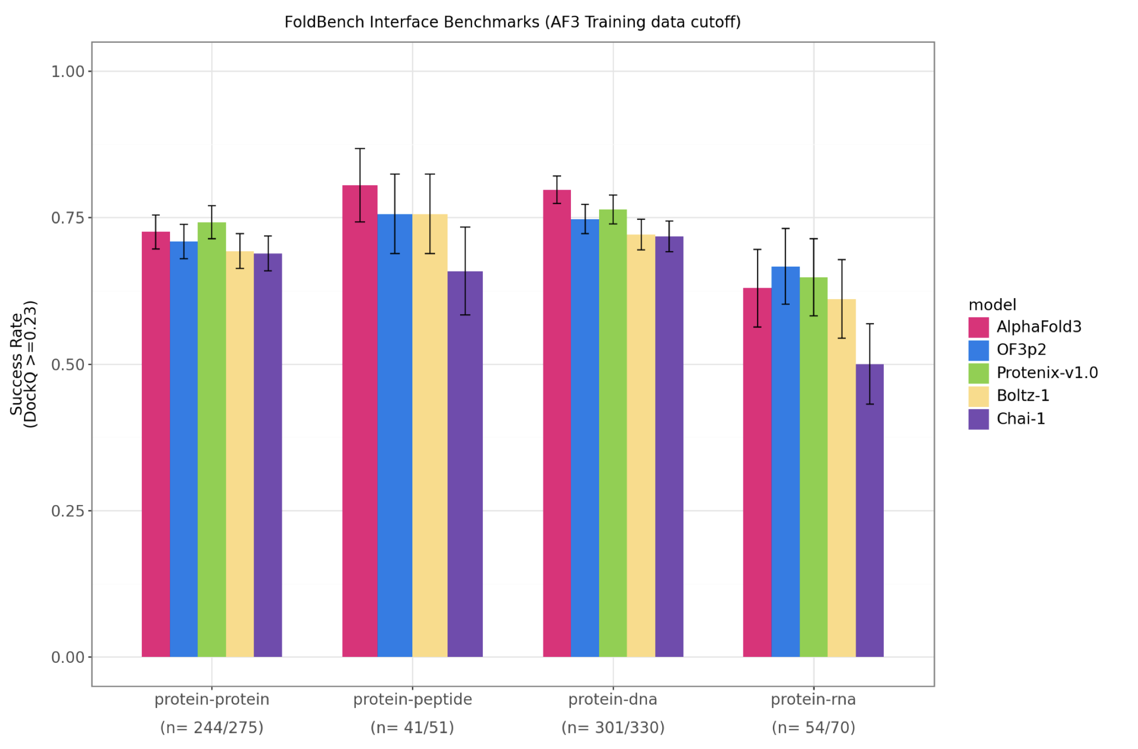
Where the MGnify distillation advantage actually shows up
One reason I am suspicious of treating MGnify as just more sequence data: the performance advantage does not appear uniformly across every interface benchmark. It shows up strongly in antibody-antigen prediction, while most of the broader cofolding benchmarks remain closer together. This is not a clean causal experiment — architecture, compute, and training details all move at once — but it fits the intuition that protein-protein interaction accuracy improves when the model has seen much more of natural protein space.
Spectral linker split
This is a standalone version of the graph split used above. It assumes
you have already filtered out low-confidence residues, and that
ca_coords contains only the C-alpha coordinates you still
want to consider. The function returns the C-alpha indices that sit
closest to Fiedler sign-change boundaries; in our pipeline those
residues become linker/cut residues before fragment IDs are assigned.
import numpy as np
from scipy.sparse import csr_matrix
from scipy.spatial import KDTree


def spectral_linker_indices(
    ca_coords: np.ndarray,
    *,
    k: int = 15,
    sigma: float = 8.0,
    connectivity_threshold: float = 0.05,
    boundary_size: int = 4,
    min_partition_size: int = 50,
) -> np.ndarray:
    """
    Find linker-like C-alpha positions with recursive spectral bisection.

    Parameters
    ----------
    ca_coords:
        Array with shape (N, 3), containing only the C-alpha coordinates that
        survived whatever filtering you want to apply first, usually pLDDT.
    k:
        Number of spatial nearest neighbors used to build the residue graph.
    sigma:
        Gaussian bandwidth for edge weights: exp(-d^2 / (2 sigma^2)).
    connectivity_threshold:
        Stop splitting when the Fiedler value is above this threshold.
    boundary_size:
        Number of residues closest to each sign-change boundary to mark.
    min_partition_size:
        Do not try to split partitions smaller than this.

    Returns
    -------
    np.ndarray
        Sorted indices into ca_coords. These are the residues to treat as
        linkers/cuts before assigning final fragments.
    """
    coords = np.asarray(ca_coords, dtype=float)
    if coords.ndim != 2 or coords.shape[1] != 3:
        raise ValueError("ca_coords must have shape (N, 3)")

    n = len(coords)
    if n < min_partition_size:
        return np.array([])

    k_eff = min(k, n - 1)
    if k_eff < 1:
        return np.array([])

    tree = KDTree(coords)
    distances, neighbors = tree.query(coords, k=k_eff + 1)

    # Skip the self-neighbor in column 0.
    row = np.repeat(np.arange(n), k_eff)
    col = neighbors[:, 1:].ravel()
    weights = np.exp(-(distances[:, 1:] ** 2).ravel() / (2 * sigma**2))

    W = csr_matrix((weights, (row, col)), shape=(n, n))
    W = W.maximum(W.T)

    linker_indices: set[int] = set()

    def split(node_indices: np.ndarray) -> None:
        if len(node_indices) < min_partition_size:
            return

        idx = np.sort(node_indices)
        sub_W = W[idx][:, idx].toarray()

        degree = sub_W.sum(axis=1)
        if np.count_nonzero(degree) < 2:
            return

        d_inv_sqrt = np.zeros_like(degree)
        nonzero = degree > 0
        d_inv_sqrt[nonzero] = 1.0 / np.sqrt(degree[nonzero])

        # Normalized graph Laplacian: L_sym = I - D^-1/2 W D^-1/2.
        L_sym = np.eye(len(idx)) - d_inv_sqrt[:, None] * sub_W * d_inv_sqrt[None, :]

        evals, evecs = np.linalg.eigh(L_sym)
        if len(evals) < 2:
            return

        fiedler_value = evals[1]
        fiedler_vector = evecs[:, 1]
        if fiedler_value > connectivity_threshold:
            return

        boundary_order = np.argsort(np.abs(fiedler_vector))[:boundary_size]
        linker_indices.update(idx[boundary_order].tolist())

        keep = np.ones(len(idx), dtype=bool)
        keep[boundary_order] = False

        partition_a = idx[keep & (fiedler_vector < 0)]
        partition_b = idx[keep & (fiedler_vector >= 0)]

        split(partition_a)
        split(partition_b)

    split(np.arange(n))
    return np.array(sorted(linker_indices))
Foldseek command
For the fragment clustering pass, this is the Foldseek command we used before the representative-level structural audit.
# Foldseek command for reproducibility
$FOLDSEEK cluster "$DB_DIR/fragDB" "$DB_DIR/fragCluDB" "$TMP_DIR" \
  --threads "$THREADS" \
  -c 0.8 --cov-mode 0 \
  --tmscore-threshold 0.7 \
  --tmscore-threshold-mode 1 \
  --lddt-threshold 0.6 \
  --max-seqs 2000 \
  -e 0.001 \
  --alignment-type 2 \
  --cluster-reassign 1 \
  -v 2
Citation
Please cite this work as:
Arda Goreci, "The Unreasonable Redundancy of Nature's Protein Folds",
Ligo Biosciences Blog, May 20, 2026.
Or use the BibTeX citation:
@article{goreci2026naturesproteinfolds,
  author = {Arda Goreci},
  title = {The Unreasonable Redundancy of Nature's Protein Folds},
  journal = {Ligo Biosciences Blog},
  year = {2026},
  month = may,
  day = {20},
  publisher = {Ligo Biosciences}
}