Each week, I send out one Python tutorial to help you get started with algorithmic trading, market data analysis, and quant finance. If you need support with code or strategy design, join our network. You’ll instantly join our group chat and get access to the code notebooks. Grab an Alpha Lab membership to get monthly backtested trading strategies.
In today’s post, you’ll compute rolling z-scores and rolling worst returns using pandas on real prices.
Rolling statistics compute a metric over a fixed window that slides forward in time to summarize recent behavior.
Early chartists used moving averages to smooth prices, and Welles Wilder popularized mechanical indicators built from rolling windows. In the 1990s, RiskMetrics spread rolling volatility and covariance estimates across banks, and modern data tools made them routine.
Today, professionals treat rolling windows as production features that drive signals and risk controls directly.
A mean reversion desk measures a rolling z-score of returns, then triggers entries when moves look statistically extreme. Risk teams monitor rolling minimum returns to size positions and to catch regimes where losses cluster.
Engineering pipelines compute these features on bar data and lag them by one period before storing alongside clean prices.
If you are new, rolling windows build intuition while producing testable, production-ready features from prices.
You will learn to detect outliers, track trend pressure, and measure risk without writing fragile loops. That translates to cleaner backtests and faster iteration because your features line up with returns by construction.
Let’s see how it works with Python.
Install the libraries needed to fetch market data, compute rolling windows, and render charts in this notebook.
yfinance pulls prices, pandas provides rolling operations on DataFrames, and matplotlib underpins pandas plotting so .plot() works without extra imports. Installing them up front reduces environment drift and makes the notebook reproducible across machines.
We use yfinance to download historical prices from Yahoo Finance; the returned pandas objects expose rolling calculations and plotting backed by matplotlib.
Keeping imports minimal helps isolate the rolling-window logic we want to learn without hiding behavior behind frameworks. Using a single data source also reduces version mismatches, which is important when you validate signals and their alignment later.
Pull a clean daily price history for NFLX over a fixed window so our rolling features have enough bars to stabilize and so results are reproducible.
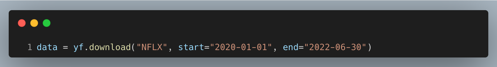
yfinance returns a pandas DataFrame with OHLCV columns; we will focus on Close for simplicity. Many production workflows prefer Adjusted Close to include corporate actions, but the rolling mechanics are identical. Working with one asset lets us focus on window alignment before scaling out.
Define a window function that scores the latest price relative to its recent history, then apply it over a 30-bar rolling window; we keep the window uncentered so it only uses information available up to the current bar.
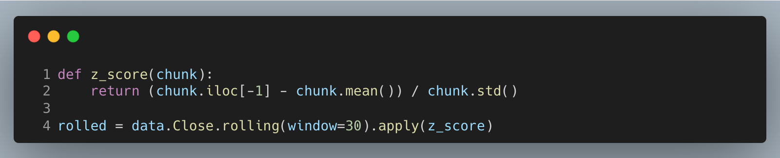
This yields a standardized feature where larger positive values mean the price sits above its recent mean by more local volatility. For backtests, join this feature to returns with a one-bar lag to avoid lookahead bias; we compute on bar t but must act on bar t+1. .apply makes the per-window logic explicit for learning, while vectorized rolling means/std are faster in production.
Compute the worst daily percentage change observed in each 30-day window to monitor downside clustering and inform risk sizing.
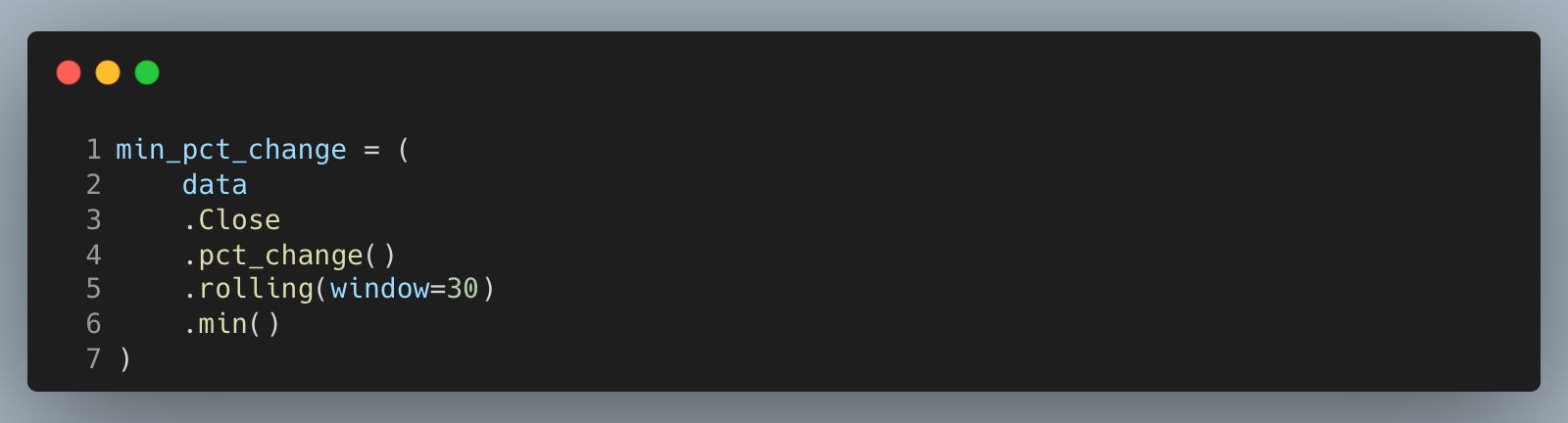
A rolling minimum of returns flags stress periods where losses accumulate and can guide position caps or de-risking rules. We compute returns first and then roll so the window advances strictly forward in time. As with the z-score, plan to lag this feature one bar before using it to drive decisions.
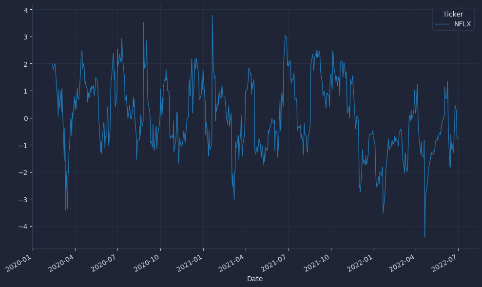
Plot time series and histograms of both features to spot alignment issues and understand distribution shape before you backtest thresholds.
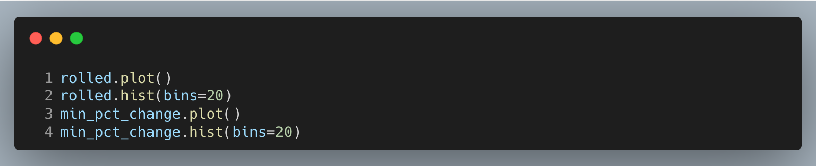
The result is a set of charts that look like this.

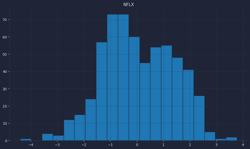
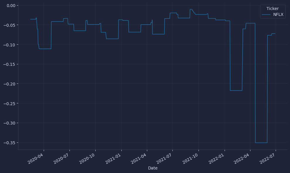
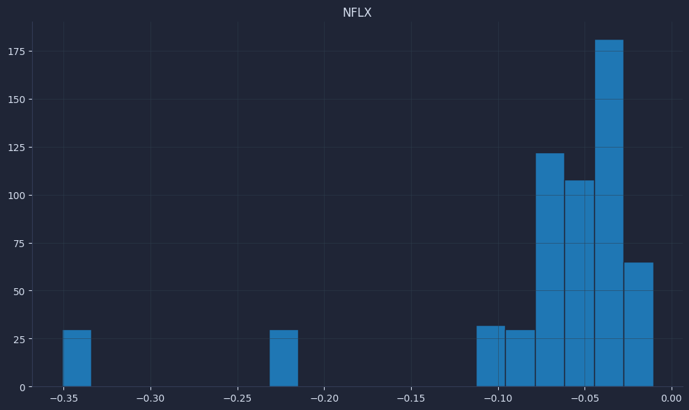
Quick visuals reveal problems like unexpected spikes or long runs of NaNs; initial values should be NaN until 30 observations accumulate, which pandas handles automatically.
Check that z-scores mostly sit in a sensible range (often within a few standard deviations) and that worst-return windows look plausible for the asset. Validating these basics now prevents quiet data leakage and miscalibrated signals later.
Now you can compute rolling z-scores and rolling worst returns on real prices in pandas, keep windows unidirectional, and lag features one bar so signals line up without leakage.
These features turn prices into testable entries and risk checks for production, improving backtest integrity, sizing, and iteration speed.