Full Code / IR Dumps: https://github.com/patrick-toulme/justabyte/tree/main/maxtext_pretraining
Connect on LinkedIn: https://www.linkedin.com/in/patrick-toulme-150b041a5/
Follow on X: https://x.com/PatrickToulme
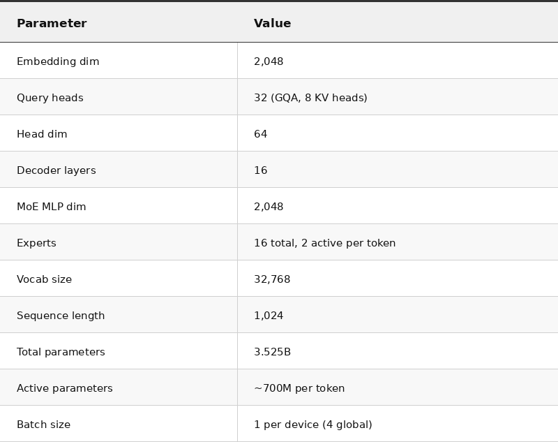
3.5 billion parameters. 16 MoE experts with top-2 routing. 2-way FSDP sharded across 2 chips, expert-parallel across the other 2 chips. 200 training steps at 22 TFLOP/s per device — every step generating 887 fused kernels, 104 async all-gathers, 12 ragged all-to-all collectives, 8 Pallas attention kernels, and 24 MegaBlox grouped matmuls. All compiled, scheduled, and overlapped automatically from a single python3 -m maxtext.trainers.pre_train.train command.
The cost of this entire experiment was under 10 dollars.
I keep watching startups, neo-frontier labs and major organizations spend months rebuilding training infrastructure from scratch in PyTorch on NVIDIA GPUs. FSDP sharding, kernel fusion, collective overlap, MoE routing. Team after team duplicating the same work, and it's not clear most of them even achieve as high an MFU as MaxText gets out of the box. Meanwhile, I rarely hear MaxText mentioned as even an option.
I’m not claiming a frontier lab can take MaxText off the shelf and ship. But I am claiming they could get to a production training job dramatically faster by building on top of it — and this post shows why. I understand some organizations have bespoke requirements or privacy reasons that prevent them from using open source — this post isn't aimed at them.
This experiment runs on 4 chips, but MaxText and JAX's SPMD model scale with no code changes. You change ici_fsdp_parallelism=2 to ici_fsdp_parallelism=128 and the same code runs on 128 chips. The compilation pipeline I traced here — the fusions, the async collectives, the VMEM scheduling — is the same compilation pipeline at any scale. The only things that change are the mesh dimensions in a config flag.
I ran a GPT-OSS MoE pretraining job on 4 TPU v6e chips, dumped the IR, and traced the full compilation pipeline from Python down to fused TPU kernels. What I found: the XLA compiler does a staggering amount of work that would take months of manual kernel engineering. The fusion, the async scheduling, the memory management, the SPMD partitioning — it’s all generated automatically. This is the infrastructure teams are rebuilding by hand.
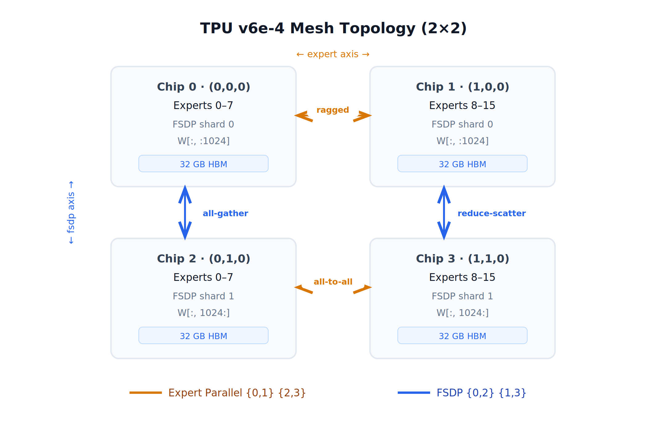
Hardware: a single TPU v6e-4 node – 4 TPU v6e chips in a 2×2 mesh, each with 32 GB HBM. Total: 128 GB HBM across the node.
[TpuDevice(id=0, coords=(0,0,0)), TpuDevice(id=1, coords=(1,0,0)),
 TpuDevice(id=2, coords=(0,1,0)), TpuDevice(id=3, coords=(1,1,0))]
Software: MaxText cloned from AI-Hypercomputer/maxtext, installed with pip install -e ".[tpu]". JAX 0.9.0, libtpu 0.0.36. Nothing else.
The model: a scaled variant of GPT-OSS (OpenAI’s recently open-sourced MoE architecture). The released gpt-oss-20b uses 32 experts with 4 active experts per token; I adjusted width/depth and used 16 experts with top-2 routing to fit on 4 chips—the point here is tracing the compiler + SPMD stack, not exact parity with the released checkpoints.
The parallelism: 2-way FSDP × Expert Parallelism-2. Weights are sharded across 2 chips (FSDP), and the 16 experts are partitioned across 2 chips (EP). This requires real multi-axis communication – all-gather for FSDP weight reconstruction and ragged all-to-all for MoE token dispatch.
python3 -m maxtext.trainers.pre_train.train src/maxtext/configs/base.yml \
  model_name="gpt-oss-20b" override_model_config=true \
  base_emb_dim=2048 base_num_decoder_layers=16 \
  num_experts=16 num_experts_per_tok=2 \
  megablox=true sparse_matmul=true capacity_factor=-1.0 \
  ici_fsdp_parallelism=2 ici_expert_parallelism=2 \
  attention='flash' remat_policy=full dtype=bfloat16 \
  dump_hlo=true dump_jaxpr=true ...
That ici_fsdp_parallelism=2 ici_expert_parallelism=2 line is the entire parallelism specification. The same codebase handles single chip debugging and multi thousand chip production training – the parallelism strategy is a configuration parameter, not code.
Note: 2-way FSDP × 2-way EP is not the most optimal parallelism configuration for this model and chip count. The point of this experiment is demonstrating the capability of the stack, not maximizing utilization or FLOP/s.
MaxText is Google’s open-source JAX/Flax training framework for large language models. It sits at AI-Hypercomputer/maxtext and is the reference implementation for training on TPUs.
The architecture has four layers:
Configuration. MaxText uses OmegaConf + Pydantic for model config. You pick a base architecture with model_name="gpt-oss-20b" (which selects the decoder layer class, attention pattern, MoE routing style) and then override any dimension with CLI flags: base_emb_dim=2048 base_num_decoder_layers=16 num_experts=16.
Model layers (Flax NNX). The model definition is pure Python using Flax’s NNX API. GptOssDecoderLayer in models/gpt_oss.py is 289 lines – it composes an Attention module, an RMSNorm, and a RoutedMoE with residual connections and dropout. The scannable block wraps multiple decoder layers with alternating attention patterns (local sliding-window, global) for nn.scan compilation.
Custom kernels (Pallas). Performance-critical operations – grouped matrix multiplication for MoE, flash attention – are hand-written Pallas kernels. Pallas is JAX’s kernel authoring language that compiles to tpu_custom_call ops. These are the only hand-written kernels in the stack; everything else is generated by XLA.
Parallelism (JAX SPMD). MaxText defines a 13-axis logical mesh (fsdp, expert, tensor, data, sequence, …) and annotates tensors with nn.with_logical_constraint. JAX’s Shardy partitioner reads these annotations and automatically inserts all-gathers, reduce-scatters, and ragged all-to-all collectives.
The key insight: MaxText is a thin layer. The model definition is high level Python. The kernels handle the MXU-level compute. Everything in between – fusion, scheduling, communication, memory management – is the compiler’s job.
step:   0, seconds: 30.309, TFLOP/s/device:  0.133, loss: 10.871  # compilation
step:   1, seconds:  0.531, TFLOP/s/device:  7.598, loss: 10.871  # warmup
step:   3, seconds:  0.182, TFLOP/s/device: 22.194, loss: 10.730  # steady state
step:  50, seconds:  0.180, TFLOP/s/device: 22.441, loss:  0.008
step: 100, seconds:  0.180, TFLOP/s/device: 22.446, loss:  0.002
step: 199, seconds:  0.180, TFLOP/s/device: 22.368, loss:  0.001
Step 0 takes 30 seconds – XLA compilation. By step 3, we’re at steady state. Note: this run uses dataset_type=synthetic, so the rapid loss collapse is expected (fast memorization). The goal is validating throughput and end-to-end correctness of MoE + collectives + optimizer, not model quality. 182 ms per step, 22.2 TFLOP/s per device, 5,640 tokens/s/device. The loss drops from 10.87 to 0.001 – synthetic data memorization confirming the full pipeline works: forward through 16 MoE layers, loss computation, backward through MegaBlox kernels and routing gradients, gradient reduce-scatter across devices, and AdamW optimizer update.
Here’s something that surprises people coming from PyTorch: the entire training step – forward pass through 16 MoE decoder layers, cross-entropy loss, backward pass through every layer including custom MegaBlox VJPs, gradient reduce-scatter across all 4 devices, and AdamW optimizer update – is compiled into a single XLA binary.
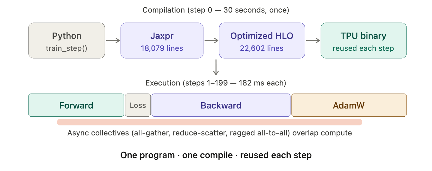
This is what @jax.jit does. When MaxText calls train_step(state, batch), JAX traces the full Python function into a Jaxpr (18,079 lines of functional IR). XLA then compiles that Jaxpr into a single HLO module (22,636 lines after optimization). That module is compiled once into a TPU binary. Every subsequent step just re-executes the same binary with new inputs.
This is why step 0 takes 30 seconds and step 1 takes 0.5 seconds. Step 0 is compilation. Steps 1-199 are execution.
The consequence: XLA sees everything at compile time. That turns the training step into one schedulable program instead of a chain of compiled islands. XLA can fuse across the forward/backward/optimizer boundary, and it can overlap communication with compute by issuing async all-gathers early and consuming them later—e.g., pulling layer 5’s shards while layer 3’s backward pass runs. With separate compilation units, those boundaries act like barriers: more launches, more forced materialization, and less automatic comm/compute overlap.
Between python3 -m maxtext.trainers.pre_train.train and the TPU executing 182 ms training steps, the code passes through four IR layers. MaxText’s dump_hlo=true and dump_jaxpr=true flags capture all of them.
JAX traces the Python training step into Jaxpr – a functional IR that captures the computation graph. Our train step produces an 18,079-line Jaxpr with 207 helper function definitions encoding the full MoE routing logic:
train_step → jit → TransformerLinenPure.apply → Decoder.__call__
  → scan (16 layers) → GptOssScannableBlock.__call__
    → GptOssDecoderLayer.__call__
      → shard_map → Attention (splash_mha Pallas kernel)
      → shard_map → RoutedMoE.__call__
        → permute → ragged_all_to_all → gmm (MegaBlox Pallas kernel) → unpermute
  → cross_entropy_with_logits
  → TrainState.apply_gradients → adam → reduce_scatter
The Jaxpr reveals the primitive inventory: 112 dot_general (matrix multiplies), 120 sharding_constraint (SPMD annotations), 32 custom_vjp_call (custom backward passes for GMM and attention), 16 shard_map (manual sharding regions), 12 pallas_call (custom TPU kernels), and 16 scan iterations.
The mesh configuration appears directly in the Jaxpr:
ctx_mesh=Mesh('diloco': 1, 'data': 1, 'stage': 1, 'fsdp': 2,
              'fsdp_transpose': 1, 'sequence': 1, 'context': 1,
              'context_autoregressive': 1, 'tensor': 1,
              'tensor_transpose': 1, 'tensor_sequence': 1,
              'expert': 2, 'autoregressive': 1)
Thirteen logical mesh axes, but only two are active: fsdp=2 and expert=2. XLA’s SPMD partitioner reads these annotations and generates all the necessary collectives.
Jaxpr lowers to HLO (High-Level Operations), XLA’s main IR. Before optimization, our train step is 14,541 lines of HLO with 11,207 individual instructions and zero fusion blocks.
This is the key: everything is separate. Every add, multiply, convert, broadcast, reduce is its own HLO instruction. Let me show you what this actually looks like.
RMSNorm – 10 separate instructions for one normalization:
%convert.105 = f32[4,1024,2048] convert(%input_bf16)           // bf16 → f32
%square.4   = f32[4,1024,2048] multiply(%convert.105, %convert.105)  // x²
%reduce.92  = f32[4,1024]      reduce(%square.4, zero), dims={2}     // Σx²
%reshape.1  = f32[4,1024,1]    reshape(%reduce.92)              // broadcast prep
%div.48     = f32[4,1024,1]    divide(%reshape.1, 2048.0)       // mean(x²)
%add.217    = f32[4,1024,1]    add(%div.48, 1e-5)               // + ε
%rsqrt.4    = f32[4,1024,1]    rsqrt(%add.217)                  // 1/√(mean(x²)+ε)
%bcast.1    = f32[4,1024,2048] broadcast(%rsqrt.4)              // expand
%mul.128    = f32[4,1024,2048] multiply(%convert.105, %bcast.1) // x * scale
%convert.106 = bf16[4,1024,2048] convert(%mul.128)              // f32 → bf16
Ten HLO instructions. Each one reads its input from HBM and writes its output back to HBM. For a f32[4,1024,2048] tensor, that’s 32 MB per read/write. This RMSNorm alone would generate 320 MB of memory traffic without fusion. There are 32 RMSNorm instances in this model (2 per layer × 16 layers).
Adam optimizer – 15 separate instructions per parameter update:
%mul.1073  = f32[2048,8] multiply(grad, 0.1)               // (1-β₁) * grad
%mul.1074  = f32[2048,8] multiply(mu_old, 0.9)             // β₁ * μ
%add.1253  = f32[2048,8] add(%mul.1073, %mul.1074)         // μ_new
%div.614   = f32[2048,8] divide(%add.1253, bias_correction) // μ̂
%pow.59    = f32[2048,8] multiply(grad, grad)               // grad²
%mul.1155  = f32[2048,8] multiply(%pow.59, 0.05)            // (1-β₂) * grad²
%mul.1156  = f32[2048,8] multiply(nu_old, 0.95)             // β₂ * ν
%add.1294  = f32[2048,8] add(%mul.1155, %mul.1156)          // ν_new
%div.696   = f32[2048,8] divide(%add.1294, bias_correction) // ν̂
%sqrt.64   = f32[2048,8] sqrt(%div.696)                     // √ν̂
%add.1336  = f32[2048,8] add(%sqrt.64, 1e-8)               // √ν̂ + ε
%div.759   = f32[2048,8] divide(%div.614, %add.1336)       // μ̂/(√ν̂+ε)
%mul.1219  = f32[2048,8] multiply(param, 0.1)               // weight decay
%add.1377  = f32[2048,8] add(%div.759, %mul.1219)          // update + WD
%add.1422  = f32[2048,8] add(param, lr * %add.1377)        // θ_new
This pattern repeats for 40+ parameter tensors. That’s 600+ element-wise HLO instructions just for the optimizer.
After XLA’s optimization passes, the picture changes dramatically:
The optimized IR is longer because XLA outlines each fused computation as a separate block, but those 11,207 individual instructions have been compressed into hundreds of fused kernels. Each fusion reads its inputs from HBM once, executes all operations in VMEM, and writes outputs once.
Let me show you what these fusions look like.
Before looking at individual fusions, here’s the full picture.
The backward pass dominates: 492 fusions vs. 274 forward. This isn’t surprising – the backward pass through MoE requires separate gmm (input gradient) and tgmm (weight gradient) kernels for each forward GMM, plus chain-rule fusions through every activation, normalization, and residual connection. The 22 backward Pallas kernels vs. 10 forward kernels reflect the same 2:1+ ratio at the custom kernel level.
The optimizer is compact – just 41 fusions – but each one is a monster. A single AdamW fusion handles gradient scaling, both moment EMAs, bias correction, weight decay, and the parameter update for an entire tensor. The L2 norm reduction for gradient clipping is fused in too.
Nearly a quarter of all fusions (188 out of 832) contain bf16↔f32 type conversions. The model computes in bf16 for throughput but accumulates in f32 for numerical stability. XLA fuses these conversions into the surrounding operations so they never hit HBM as separate ops.
Now let me show you what these fusions look like in practice.
This is where XLA goes beyond element-wise fusion. The forward logits computation – RMSNorm scaling, the [1024,2048] × [2048,32768] matmul into vocabulary space, and the reduce_max for softmax numerical stability – all in a single kOutput fusion:
%fused_computation.1802 (weights: bf16[2048,32768],
    norm_weight: bf16[2048], rsqrt_scale: f32[1024],
    activation: bf16[1,1024,2048])
    -> (bf16[1024], bf16[1024,32768]) {
  // RMSNorm: scale activation (nested kLoop fusion)
  %normed    = fusion(norm_weight, rsqrt_scale, activation)  // bf16[1024,2048]
  %w_reshaped = fusion(weights)                               // layout bitcast

  // THE MATMUL: [1024,2048] × [2048,32768] → logits
  %logits    = bf16[1024,32768] convolution(%normed, %w_reshaped),
                 dim_labels=bf_io->bf                         // logits_dense forward

  // FUSED: reduce_max over vocab dim (softmax numerics)
  %row_max   = bf16[1024] reduce(%logits, -inf), dimensions={1}

  ROOT tuple(%row_max, %logits)
}
The reduce_max consumes logits tiles as the convolution (matmul) produces them – the full bf16[1024,32768] tensor (64 MB) never needs a separate read pass. In the unfused version, XLA would write the logits to HBM, then read them back for the max. The kind=kOutput annotation means this fusion is anchored on the convolution – XLA built the fusion outward from the matmul, pulling in both its input preparation (RMSNorm) and its consumer (reduce_max).
The backward pass shows an even deeper kOutput fusion. The gradient flows backward through the logits projection and directly into the RMSNorm gradient – matmul and normalization backward fused into one kernel:
%fused_computation.1488 (activation: bf16[1,1024,2048],
    norm_weight: bf16[2048], weights: bf16[2048,32768],
    dLogits: bf16[1024,32768], row_max: f32[1024],
    softmax_denom: f32[1024], labels: bf16[1024],
    label_indices: s32[1024], loss_scale: f32[1024])
    -> (f32[1024], bf16[1024,2048]) {
  // Softmax gradient correction (nested kLoop fusion)
  %dLogits_corrected = fusion(dLogits, row_max, softmax_denom,
                              labels, label_indices, loss_scale)  // bf16[1024,32768]

  // THE MATMUL: dLogits × W^T → dActivation
  %dAct      = bf16[1024,2048] convolution(%dLogits_corrected, weights),
                 dim_labels=bf_oi->bf                     // backward logits_dense

  // FUSED: RMSNorm backward -- no HBM round-trip after matmul
  %scaled    = bf16[1,1024,2048] multiply(bitcast(%dAct), broadcast(norm_weight))
  %f32_grad  = f32[1,1024,2048] convert(%scaled)         // bf16 → f32
  %f32_act   = f32[1,1024,2048] convert(activation)      // bf16 → f32
  %chain     = f32[1,1024,2048] multiply(%f32_act, %f32_grad)  // chain rule
  %grad_sum  = f32[1024] reduce(%chain, 0.0), dimensions={0,2} // RMSNorm weight grad

  ROOT tuple(%grad_sum, %dAct)
}
The [1024,32768] × [32768,2048] backward matmul produces dAct, which is immediately consumed by the RMSNorm gradient chain: scale by norm weight, convert bf16→f32, elementwise multiply with saved activations, reduce-sum over hidden dim. Seven operations after the matmul, all executing on the convolution’s output tiles without an HBM round-trip. That’s 64 MB of avoided intermediate traffic for the matmul output alone.
The deepest matmul fusion in the model. Inside the decoder backward pass, XLA fuses a 32-head grouped convolution with residual gradient accumulation and the full RMSNorm backward chain:
%fused_computation.372 (saved_activations: bf16[8,1,1024,2048],
    layer_idx: s32[], norm_weight: bf16[2048],
    O_weight: bf16[1,2048,32,64],
    dQ_heads: bf16[1,1024,32,32], dK_heads: bf16[1,1024,32,32],
    residual_grad_1: bf16[1024,2048,1],
    residual_grad_2: bf16[1024,2048,1])
    -> (f32[1024], bf16[1024,2048]) {
  // Extract this layer's activations from scan buffer
  %act_slice  = dynamic-slice(saved_activations, layer_idx, 0, 0, 0)  // bf16[1,1024,2048]
  %f32_act    = f32[1,1024,2048] convert(%act_slice)                   // bf16 → f32

  // Accumulate two residual gradient streams
  %residual   = bf16[1024,2048] add(residual_grad_1, residual_grad_2)

  // Prepare attention head gradients and weights
  %dHeads     = fusion(dQ_heads, dK_heads)         // bf16[1024,32,64]: merged Q+K grads
  %W_reshaped = fusion(O_weight)                   // bf16[2048,32,64]: reshaped O projection

  // THE MATMUL: 32-head grouped attention projection backward
  %dHidden    = bf16[1024,2048,1] convolution(%dHeads, %W_reshaped),
                  window={size=32}, dim_labels=b0f_o0i->bf0       // 32 attention heads

  // Add matmul result to residual chain
  %combined   = bf16[1024,2048] add(%residual, bitcast(%dHidden))

  // RMSNorm backward: scale, convert, chain-rule multiply, reduce
  %scaled     = bf16[1,1024,2048] multiply(bitcast(%combined), broadcast(norm_weight))
  %f32_grad   = f32[1,1024,2048] convert(%scaled)                 // bf16 → f32
  %chain      = f32[1,1024,2048] multiply(%f32_act, %f32_grad)    // chain rule
  %grad_sum   = f32[1024] reduce(%chain, 0.0), dimensions={0,2}   // RMSNorm weight grad

  ROOT tuple(%grad_sum, %combined)
}
Count the operations: dynamic-slice from the scan buffer, bf16→f32 convert, two residual adds, a 32-head grouped convolution (window={size=32} – this is how TPU HLO represents grouped matmuls), broadcast, multiply, bf16→f32 convert, multiply, reduce-sum. ~20 operations across three distinct algorithmic stages (residual accumulation, attention projection, normalization backward) in a single kernel. The dynamic-slice indexed by layer_idx is particularly notable – this fusion runs inside the scan while-loop, extracting per-layer activations from the recomputation buffer each iteration.
The entire AdamW optimizer step for a single MoE expert weight tensor – gradient clipping, both moment EMAs, bias correction, weight decay, parameter update, and L2 norm computation – all in one fusion:
%fused_computation.1373 (weight: f32[8,8,2048,1024],
    lr: f32[], beta1_correction: f32[], beta2_correction: f32[],
    nu_prev: f32[8,8,2048,1024], grad_scale: f32[],
    mu_prev: f32[8,8,2048,1024], is_finite: pred[],
    gradient: f32[8,8,2048,1024])
    -> (f32[], f32[...], f32[...], f32[...], f32[]) {
  // Gradient clipping: zero out if non-finite, else scale
  %scaled_grad = divide(gradient, grad_scale)
  %safe_grad   = select(is_finite, %scaled_grad, gradient)
  // First moment: μ_t = 0.9·μ_{t-1} + 0.1·g
  %mu_new      = add(multiply(%safe_grad, 0.1), multiply(mu_prev, 0.9))
  // Second moment: ν_t = 0.95·ν_{t-1} + 0.05·g²
  %grad_sq     = multiply(%safe_grad, %safe_grad)
  %nu_new      = add(multiply(%grad_sq, 0.05), multiply(nu_prev, 0.95))
  // Bias-corrected update: μ̂/(√ν̂ + ε)
  %nu_hat      = divide(%nu_new, beta2_correction)
  %update      = divide(%mu_new, multiply(beta1_correction, add(sqrt(%nu_hat), 1e-8)))
  // Weight decay + parameter update
  %new_w       = add(weight, multiply(lr, add(%update, multiply(weight, 0.1))))
  // L2 norms for gradient clipping and logging
  %w_norm      = reduce(multiply(%new_w, %new_w), dims={0,1,2,3})
  %g_norm      = reduce(%grad_sq, dims={0,1,2,3})

  ROOT tuple(%w_norm, %new_w, %nu_new, %mu_new, %g_norm)
}
The tensor shape f32[8,8,2048,1024] is an MoE expert weight: [num_experts=8, layers_per_scan=8, hidden=2048, ffn=1024]. That’s a 512 MiB tensor. Without fusion, the 15+ intermediate reads and writes would generate ~8 GB of HBM traffic per parameter update. With fusion, it’s three reads (weight, gradient, both moments) and three writes (new weight, new μ, new ν). Two full reductions (weight norm, gradient norm) are computed in the same pass. This pattern repeats for every parameter in the model.
This is the most complex part of the compilation pipeline. The MoE layer transforms from ~500 lines of Python into a choreographed sequence of sorts, collectives, and Pallas kernels that spans all 4 TPU chips simultaneously.
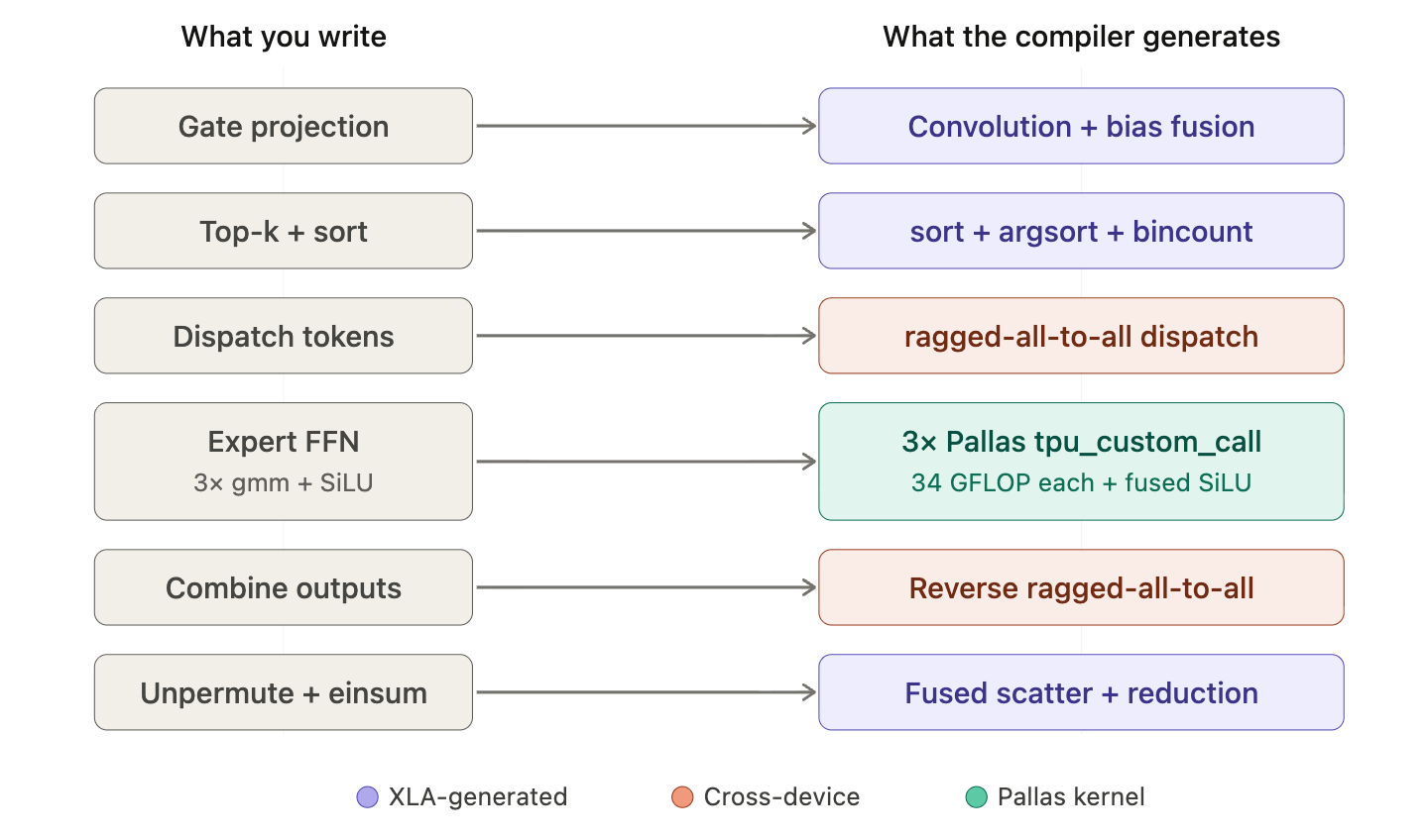
The MoE forward pass in MaxText (layers/moe.py) follows this flow:
# 1. Gate: project to expert logits
gate_logits = self.gate(inputs)                    # [batch, seq, num_experts]
top_k_weights, top_k_indices = jax.lax.top_k(gate_logits, k=2)
top_k_weights = jax.nn.softmax(top_k_weights)

# 2. Permute: sort tokens by assigned expert
sorted_inputs = _sort_activations(inputs, argsort(experts))
group_sizes = jnp.bincount(experts, length=num_experts)

# 3. Dispatch: send tokens to expert-owning devices
x = jax.lax.ragged_all_to_all(sorted_inputs, offsets, sizes, ...)

# 4. Expert FFN: three grouped matrix multiplies
gate_out = gmm(x, w0, group_sizes, tiling=(512,1024,1024))  # gate proj
up_out   = gmm(x, w1, group_sizes, tiling=(512,1024,1024))  # up proj
hidden   = silu(gate_out) * (up_out + 1)                     # activation
output   = gmm(hidden, wo, group_sizes, tiling=(512,1024,1024))  # down proj

# 5. Combine: send results back and weight-sum
x = jax.lax.ragged_all_to_all(output, ...)         # reverse dispatch
output = unpermute(x, argsort(experts))
result = einsum("BKE,BK->BE", output, weights)     # weighted combination
The gmm function wraps a Pallas kernel with a custom VJP: _gmm_fwd calls the kernel for the forward pass, _gmm_bwd calls gmm with transpose_rhs=True for the input gradient and tgmm (a separate kernel) for the weight gradient. Three different tiling configurations optimize each independently.
The shard_map wrapper around this code gives each device a local view, and ragged_all_to_all – a JAX primitive – handles the variable-length token shuffle: each device sends different numbers of tokens to each peer based on the routing decisions.
Here’s what the MoE pipeline looks like in the optimized HLO. I’ve annotated each step:
Step 1 – Token routing (sort by expert):
%sort.508 = (s32[2048], s32[2048]) sort(%experts, %iota), dimensions={0}, is_stable=trueStep 2 – Sort activations to match expert ordering:
%gather_custom_fusion.263 = bf16[2048,2048] fusion(%activations, %sort_indices)Step 3 – Dispatch tokens via ragged all-to-all:
%ragged_all_to_all.295 = bf16[4096,2,1024] ragged-all-to-all(
    %sorted_tokens,       // bf16[2048,2,1024]: local tokens
    %output_buffer,       // bf16[4096,2,1024]: receive buffer (2x for worst case)
    %send_sizes,          // s32[2]: how many tokens to send to each peer
    %send_offsets,        // s32[2]: where they start in my buffer
    %recv_sizes,          // s32[2]: how many I'll receive from each peer
    %recv_offsets),       // s32[2]: where to put them
    channel_id=1,
    replica_groups={{0,1},{2,3}}
The replica groups {{0,1},{2,3}} show the expert-parallel communication pattern: chips 0↔1 and 2↔3 exchange tokens along the expert axis of the 2×2 mesh.
Step 4 – GMM forward (Pallas custom call):
%gmm.1 = bf16[4096,2048] custom-call(
    %group_index,           // s32[]: scalar loop state
    %group_sizes,           // s32[9]: tokens per expert (+padding)
    %group_offsets_lhs,     // s32[15]: tile boundary metadata
    %group_offsets_rhs,     // s32[15]: tile boundary metadata
    %num_actual_groups,     // s32[1]: 8 experts per shard
    %dispatched_tokens,     // bf16[4096,2048]: sorted tokens (LHS)
    %expert_weights),       // bf16[8,2048,2048]: expert matrices (RHS)
    custom_call_target="tpu_custom_call",
    kernel_metadata={"tiling": {"tile_m": 512, "tile_k": 1024, "tile_n": 1024},
                     "cost_estimate": {"flops": "34359738368"}}
Each GMM call does ~34.4 GFLOP – tiling [512, 1024, 1024] across the M (token), K (input), and N (output) dimensions. The group metadata tells the kernel where each expert’s tokens start and end in the sorted input.
Step 5 – SiLU activation (fused into a single kernel):
%fusion.1232 = bf16[4096,2048] fusion(%gmm.0, %gmm_shuffled, %gmm.1, %weights),
    kind=kLoop, calls=%fused_computation.341   // ← the SiLU fusion shown earlier
Step 6 – Combine via reverse ragged all-to-all back to original device mapping.
Inside the tpu_custom_call, the Pallas GMM kernel runs on a 3D grid (tiles_n, num_active_tiles, tiles_k):
grid=(tiles_n, num_active_tiles, tiles_k)
# tiles_n=2:      N-dimension tiles (parallel)
# num_active_tiles: M-tiles covering all groups (sequential)
# tiles_k=2:      K-dimension accumulation (sequential)
The first dimension is marked "parallel" – independent axis. The kernel body:
Fetch: DMA a
[512, 1024]tile of sorted tokens from HBM to VMEMFetch: DMA the correct expert’s
[1024, 1024]weight tile (selected bygroup_ids[grid_id])Accumulate:
acc_scratch += dot(lhs_tile, rhs_tile)in VMEM f32 scratchOn last k-tile: Apply group boundary mask and store result to HBM
The boundary mask handles the case where a single tile spans two experts: only rows belonging to the current expert are written.
The backward pass through MoE requires custom VJPs at the ops.py level. For each of the three forward GMM calls:
gmmwithtranspose_rhs=Truecomputes∂L/∂input = grad @ W^T– the input activation gradienttgmmcomputes∂L/∂W = input^T @ grad– the weight gradient
The tgmm kernel has a fundamentally different structure: it produces [num_experts, K, N] output, detecting group boundaries to accumulate then store per-expert weight gradients. Its Pallas grid is (tiles_n, tiles_k, num_active_tiles) – note the reordered axes.
In the optimized HLO, you can see both:
// Input gradient: gmm with transposed weights
%gmm.10 = bf16[4096,2048] custom-call(..., %expert_weights), target="tpu_custom_call"

// Weight gradient: tgmm (separate kernel body)
%tgmm.2 = bf16[8,2048,2048] custom-call(
    ..., %saved_activations, %upstream_grad), target="tpu_custom_call",
    kernel_metadata={"tiling": {"tile_m": 512, "tile_k": 1024, "tile_n": 1024},
                     "num_actual_groups": 8}
The 2×2 mesh creates three distinct communication topologies, all visible in the IR. In total: 104 async all-gathers, 12 ragged all-to-all, 10 plain all-to-all, 8 reduce-scatters, and 22 all-reduces – 156 collective operations in a single training step.
This is the most sophisticated pattern. XLA doesn’t just make all-gathers async – it fuses them with compute into a single pipelined operation. While the current layer’s backward matmul runs, the all-gather for the next layer’s FSDP-sharded weights is in flight:
%async_collective_fusion.1497 (
    shard: bf16[1,8,2048,1024],     // FSDP-sharded expert weight (half)
    full_weight: bf16[1,8,2048,2048],  // previous all-gather result
    semaphore: s32[2],              // collective sync state
    flags: u32[], u32[], ...,       // S(2) flag registers
    gate_bias: bf16[16],            // router bias
    gate_weight: bf16[1,2048,16],   // router projection
    activation: bf16[1024,2048])    // layer input
    -> (bf16[1,1024,16], ..., bf16[1,8,2048,2048], ...) {

  // ===== COMPUTE: router backward matmul =====
  %dGate   = bf16[1024,16] convolution(activation, gate_weight),
               dim_labels=bf_io->bf                    // [1024,2048] × [2048,16]
  %dGate   = add(bitcast(%dGate), broadcast(gate_bias))  // + bias

  // ===== COMMS: all-gather for NEXT layer (overlapped) =====
  %gathered = bf16[1,8,2048,2048] all-gather(shard),
               channel_id=38,
               replica_groups=[2,2]<=[2,2]T(1,0),      // FSDP: {0,2},{1,3}
               dimensions={3},                          // double dim 3: 1024 → 2048
               frontend_attributes={chain_id="4"},      // pipeline ordering
               backend_config={async_collective_fusion_config:
                 {flag_start:"2", flag_end:"8"}}        // semaphore window

  ROOT tuple(%dGate, shard, full_weight, %gathered, semaphore, flags...)
}
The chain_id="4" and flag_start/flag_end annotations reveal XLA’s double-buffered all-gather pipeline: chain IDs sequence the all-gathers across layers, and flag registers manage the handoff between pipeline stages. The semaphore state (s32[2] in memory space S(4)) and flag registers (u32[] in S(2)) are threaded through the tuple output as “continuation state” – passed from one async collective fusion to the next.
There are 39 async collective fusions in total, wrapping 104 individual all-gather operations. The replica_groups=[2,2]<=[2,2]T(1,0) pattern (39 all-gathers) reconstructs FSDP-sharded weights across chips {0,2} and {1,3}. The [1,4]<=[4] pattern (65 all-gathers) gathers across all 4 chips for activations and non-expert parameters.
Expert parallelism uses ragged_all_to_all with variable length messages – each device sends different numbers of tokens to each peer depending on the routing decisions:
%ragged_all_to_all.295 = bf16[4096,2,1024]
    ragged-all-to-all(
        %sorted_tokens,       // bf16[2048,2,1024]: local tokens (input)
        %output_buffer,       // bf16[4096,2,1024]: receive buffer (zeros)
        %send_sizes,          // s32[2]: how many tokens to send each peer
        %recv_sizes,          // s32[2]: how many I'll receive
        %send_offsets,        // s32[2]: where they start in my buffer
        %recv_offsets),       // s32[2]: where to put them
    channel_id=1, replica_groups={{0,1},{2,3}},
    barrier_config={"barrier_type":"CUSTOM","id":"3"}
The replica groups {{0,1},{2,3}} show the expert-parallel topology: chips 0↔1 and 2↔3 exchange tokens along the horizontal axis of the 2×2 mesh. There are 12 ragged all-to-all operations (4 forward dispatch + 4 forward combine + 4 backward), plus 8 plain all-to-all exchanging small s32[2,1,1] metadata tensors for token count coordination.
The output lands in S(1) (VMEM) – dispatched tokens go straight to on-chip memory, avoiding an HBM round-trip before the GMM kernels consume them.
After the backward pass, gradients are reduce-scattered back to FSDP-sharded form. XLA batches 10 parameter gradients from 2 transformer layers into a single collective:
%all-reduce-scatter.17 (
    Q_grad:    bf16[2048,8,64],    // Q projection (layer A)
    K_grad:    bf16[32,64,2048],   // K projection (layer A)
    V_grad:    bf16[2048,32,64],   // V projection (layer A)
    O_grad:    bf16[2048,8,64],    // output projection (layer A)
    gate_grad: bf16[2048,16],      // router gate (layer A)
    Q_grad_B:  bf16[2048,8,64],    // Q projection (layer B)
    K_grad_B:  bf16[32,64,2048],   // K projection (layer B)
    V_grad_B:  bf16[2048,32,64],   // V projection (layer B)
    O_grad_B:  bf16[2048,8,64],    // output projection (layer B)
    gate_grad_B: bf16[2048,16])    // router gate (layer B)
    → (bf16[512,8,64], bf16[32,64,512], ...) {
  // All-reduce across all 4 devices, then scatter via partition-id indexing
  %all-reduce = all-reduce(inputs...), replica_groups={{0,1,2,3}}
  // Each device slices its 1/4 shard: dynamic-slice(..., partition_id * 512, ...)
}
Ten gradient tensors, one collective launch. Each output is scattered from 2048 down to 512 along the FSDP dimension via dynamic-slice indexed by partition-id. For MoE expert weights, separate reduce-scatters operate along the FSDP axis only (replica_groups={{0,2},{1,3}}).
These patterns reveal a tension in the compiler’s scheduling strategy. Coalescing wants to batch collectives together – the 10 input reduce-scatter amortizes launch overhead by waiting until all 10 gradient tensors from 2 layers are ready, then issuing one large collective instead of 10 small ones. Overlap wants to start collectives as early as possible – the async collective fusions issue all-gathers for layer N+1 while layer N’s compute is still running, hiding latency behind useful work.
XLA makes different choices for different collective types. All-gathers are overlap optimized: each weight gather launches individually inside its own async collective fusion, pipelined with chain_id ordering, because waiting to batch them would stall the compute pipeline. Reduce-scatters are coalescing optimized: batching 10 gradients into one call is worth the delay because the gradients aren’t needed until the optimizer runs, so there’s no compute to overlap them with anyway. Ragged all-to-alls are neither – they’re synchronous barriers because the MoE routing decisions create data-dependent communication patterns that can’t be predicted at compile time.
The scheduler is balancing three constraints: minimize collective launch overhead (coalesce), maximize compute-comms overlap (pipeline early), and respect data dependencies (barrier where required). The fact that it makes different choices for all-gather vs. reduce-scatter vs. ragged all-to-all shows this isn’t a one size fits all heuristic – it’s a per collective scheduling decision informed by the dependency graph.
This is the infrastructure teams are reimplementing when they rebuild training stacks from scratch. Let me quantify it.
Kernels you’d need to write: The hand-written kernel count alone is significant: 9 for MoE (gate projection, top-k selection, argsort, bincount, GMM forward, gated activation, GMM backward, TGMM for weight gradients, and unsort/combine) and 3 for attention (forward, dQ backward, dKV backward). Each needs its own tiling strategy, VMEM allocation, and DMA scheduling. But that's just the custom kernels — it doesn't include RMSNorm, softmax, embedding, cross-entropy, residual connections, or the AdamW optimizer. On TPU, XLA generates fused kernels for all of those automatically. On a from scratch PyTorch stack, you're writing or tuning those too.
Memory management decisions: ~8 critical choices. VMEM scratch allocation for GMM accumulators. HBM buffer sizing for ragged all-to-all (worst case capacity). Double-buffering strategy for weight prefetch. Activation checkpointing (MaxText uses remat_policy=full – all activations recomputed in backward). Padding strategies for tile boundaries. When to materialize vs. recompute intermediate results.
Communication patterns: ~6 distinct collective types. Ragged all-to-all for MoE dispatch (variable-length). Ragged all-to-all for MoE combine (reverse direction). FSDP all-gather for weight reconstruction. All-gather for routing metadata. Reduce-scatter for gradient sharding. All-reduce for loss aggregation. Each one needs to be overlapped with compute for efficiency.
Custom backward passes: The MoE routing sort requires a custom VJP (_sort_activations_custom_bwd) because JAX’s automatic backward for indexing is inefficient. The GMM needs separate forward/backward kernel implementations. The attention uses three different Pallas kernels for forward, dQ, and dKV.
Interacting parallelism dimensions: FSDP weight sharding, expert partitioning, and data parallelism interact in subtle ways. The weight_gather_axes logic in moe.py handles cases where weights are sharded across FSDP and must be all-gathered before GMM but reduce-scattered in backward.
The MaxText/JAX/XLA stack automates all of this. The developer writes ~500 lines of high-level Python (the RoutedMoE class) and the GMM kernel interface (282 lines). The compiler generates the remaining equivalent of ~50,000+ lines of kernel code, memory management, and communication scheduling.
The numbers tell the story: 11,207 individual HLO instructions compressed into 887 fused kernels. 39 async collective fusions containing 104 all-gathers with compute overlap. 12 ragged all-to-all collectives. 156 total collective operations. 8 Splash Attention calls and 24 GMM calls – the only handwritten code in the entire pipeline. XLA generated everything else.
This entire pretraining run — MoE architecture, Pallas kernels, XLA compilation, multi-axis SPMD sharding, async collective overlap — is open source. Every file is at AI-Hypercomputer/maxtext. The model definition: 289 lines of Python. The MoE layer: layers/moe.py. The MegaBlox kernel: 282 lines.
Out of the 22,636 lines of optimized HLO, only the Splash Attention and MegaBlox GMM calls are handwritten kernels. Everything else — 887 fused kernels, 39 async collective fusions wrapping 104 all-gathers, ~960 prefetch operations across 4 memory spaces, the entire SPMD partitioning — is generated by XLA from high level JAX code.
This is what I keep watching teams spend months rebuilding by hand. FSDP overlap, kernel fusion, MoE routing, collective scheduling — the compiler already does it, and it’s already open source. I’m not claiming a frontier lab can take MaxText off the shelf and ship tomorrow. But the distance between this codebase and a production training job is months shorter than starting from scratch on a custom PyTorch stack — and the MFU you get out of the box is likely higher than what most teams achieve after those months of work.
MaxText isn’t a ceiling — it’s a floor, and the floor is already really good. If you’re a frontier lab, you could rent V7 pods, fork MaxText, and have an MoE training loop running at high MFU before your PyTorch team finishes writing their first custom kernel. And if XLA’s codegen isn’t enough for a specific op, you write a Pallas kernel for that op — the same way Splash Attention and MegaBlox already exist in the stack. You’re not replacing the compiler; you’re surgically overriding it where it matters.
The architecture, the kernels, the compiler flags, the SPMD partitioning — it’s all the same code. The only difference between this experiment and a production training run is the number of chips.
# Clone and install (requires Python 3.12+)
git clone https://github.com/AI-Hypercomputer/maxtext.git
cd maxtext && pip install -e ".[tpu]"

# Set dump flags
export DECOUPLE_GCLOUD=TRUE
export XLA_FLAGS="--xla_dump_to=/tmp/xla_dump \
  --xla_dump_hlo_module_re=jit_train_step \
  --xla_dump_hlo_as_text --xla_dump_hlo_as_proto"
export LIBTPU_INIT_ARGS=" \
  --xla_tpu_enable_async_collective_fusion=true \
  --xla_tpu_enable_async_collective_fusion_fuse_all_gather=true \
  --xla_tpu_enable_async_collective_fusion_multiple_steps=true \
  --xla_enable_async_all_gather=true \
  --xla_tpu_overlap_compute_collective_tc=true \
  --xla_tpu_scoped_vmem_limit_kib=98304 \
  --xla_tpu_enable_data_parallel_all_reduce_opt=true \
  --xla_tpu_data_parallel_opt_different_sized_ops=true"

# Train (adjust for your chip count)
python3 -m maxtext.trainers.pre_train.train \
  src/maxtext/configs/base.yml \
  model_name="gpt-oss-20b" override_model_config=true \
  dataset_type=synthetic steps=200 \
  base_emb_dim=2048 base_num_decoder_layers=16 \
  base_num_query_heads=32 base_num_kv_heads=8 head_dim=64 \
  base_mlp_dim=2048 base_moe_mlp_dim=2048 \
  num_experts=16 num_experts_per_tok=2 \
  megablox=true sparse_matmul=true capacity_factor=-1.0 \
  per_device_batch_size=1 max_target_length=1024 vocab_size=32768 \
  attention='flash' sa_block_q=512 \
  ici_fsdp_parallelism=2 ici_expert_parallelism=2 \
  remat_policy=full enable_checkpointing=false reuse_example_batch=1 \
  base_output_directory=/tmp/maxtext_output run_name=gpt_oss_3b \
  dump_hlo=true dump_hlo_local_dir=/tmp/hlo_dumps \
  dump_jaxpr=true dump_jaxpr_local_dir=/tmp/jaxpr_dumps \
  gcs_metrics=false

# Examine the IR
ls /tmp/xla_dump/  # HLO before/after optimization
wc -l /tmp/xla_dump/*after_optimizations.txt
grep -c 'fusion' /tmp/xla_dump/*after_optimizations.txt
The IR dumps, training scripts, and full logs from this experiment are at https://github.com/patrick-toulme/justabyte.
If you found this useful, subscribe to Just a Byte for more deep dives into AI compilers, silicon, and systems.
Connect with me on LinkedIn.