(If you want to skip to the main results, you can start from Stage 2. Modeling section. My conclusions are in the last section of this post)
In the previous post, I described my desire to test the hype around Tabular Foundation Models (TFMs). In this post, you will see that I chose violence.
Of course, there are easier places to start than insurance pricing. But insurance pricing is what happens when tabular ML grows up, gets regulated, and develops a low tolerance for nonsense. The metric isn’t RMSE - it’s Tweedie deviance, or Poisson deviance, or whatever the chief actuary fought the CFO over last quarter. The model can be a single regressor - but it’s often a two-stage frequency-severity beast, or a GLM with an offset term that nobody outside the industry uses. The deployment isn’t “ship the pickle” - it’s “explain every premium change to a regulator who has a law degree and is having a rough Thursday.”
One disclaimer before we start, because I think it matters. This post will contain moments where TabPFN does not look particularly well. I want to be very clear up front: the goal here is not to dunk on TabPFN. Prior Labs is doing real research, TabPFN 3.0 is the best open TFM available right now, and if I picked the weakest model in the category, the post would be both boring and dishonest. When I find rough edges, they are almost always structural properties of the TFM paradigm itself - things that any TFM using in-context learning will run into - not a TabPFN skill issue. I’ll flag which is which as we go.
Explanation of this image will be down below, keep reading
Model: TabPFN 3.0 OSS (current release). A closed-source version of TabPFN or TFMs from contenders like Fundamental are reportedly stronger, but I don’t have access to their frontier models.
Baselines: XGBoost and LightGBM with Optuna tuning and native Tweedie objectives. GLMs (Poisson, Gamma, Tweedie) - as the industry-standard baseline. The goal is to compare TabPFN against what a competent practitioner would actually deploy - not to bury it under fifteen models.
Dataset: freMTPL2. ~670K French motor third-party liability policies. The actuarial benchmark dataset.
Workflow: Every model runs on raw features, GLM-style engineered features, and tree-friendly engineered features. I evaluate on five metrics. Then I do two things that almost nobody in the TFM discourse does: I run a competitive pricing auction to translate model quality into dollar values, and I compute SHAP values for both TabPFN and XGBoost to see whether their explanations agree.
Success Criteria: Understand scenarios where a practitioner should be using TFMs over traditional approaches
Code - in footnotes1
I always see these ML models and algorithms as merely tools - you can be very good at using a screwdriver to hammer nails - so good that using the hammer might give worse results, at least at your first try. In this case, it makes zero sense for you to do hammer benchmarking until you are comfortable. So, in an ideal benchmarking scenario set up, you would need two experts - one in traditional ML, another in TFM of choice - you lock them in separate dark rooms for a week, make them do their best, and compare the results. And do it 1000 times across different datasets and domains. Unfortunately for us, all the ML experts are now tuning their agentic systems to answer users’ queries like “summarize this email for me”. But we will do our best to set up the experiment, and I will explain how.
The modeling approaches. Insurance practitioners don’t just “predict a number.” They predict it in one of a few structurally different ways, and the choice matters.
Pure premium (single-stage). Predict expected loss per policy directly, using a Tweedie distribution that naturally handles the zero-inflation (most policies have no claims) and the right-skewed tail (the ones that do can be expensive). This is the modern actuarial default.
Frequency - severity (two-stage). Predict how often claims happen (Poisson), predict how bad they are when they happen (Gamma), multiply. This is the classical approach, and it’s still how many production systems are built.
Hurdle (two-stage, but classification). Predict whether a claim happens at all (binary classification), then predict severity given a claim occurred. I went with this instead of pure frequency because only 0.2% of freMTPL2 policies have more than one claim - so “how many claims” is mostly “did a claim happen, yes or no.” A hurdle is the simplified but honest version of the problem.
I tested the first and the last approaches. This matters for TabPFN specifically because a single-stage Tweedie model places maximum pressure on the loss function (TabPFN doesn’t optimize Tweedie), whereas a hurdle model lets you decompose the problem into pieces that TabPFN is better suited for (classification and a more well-behaved regression). I could test frequency-severity, but after the other two, it was very clear where we are.
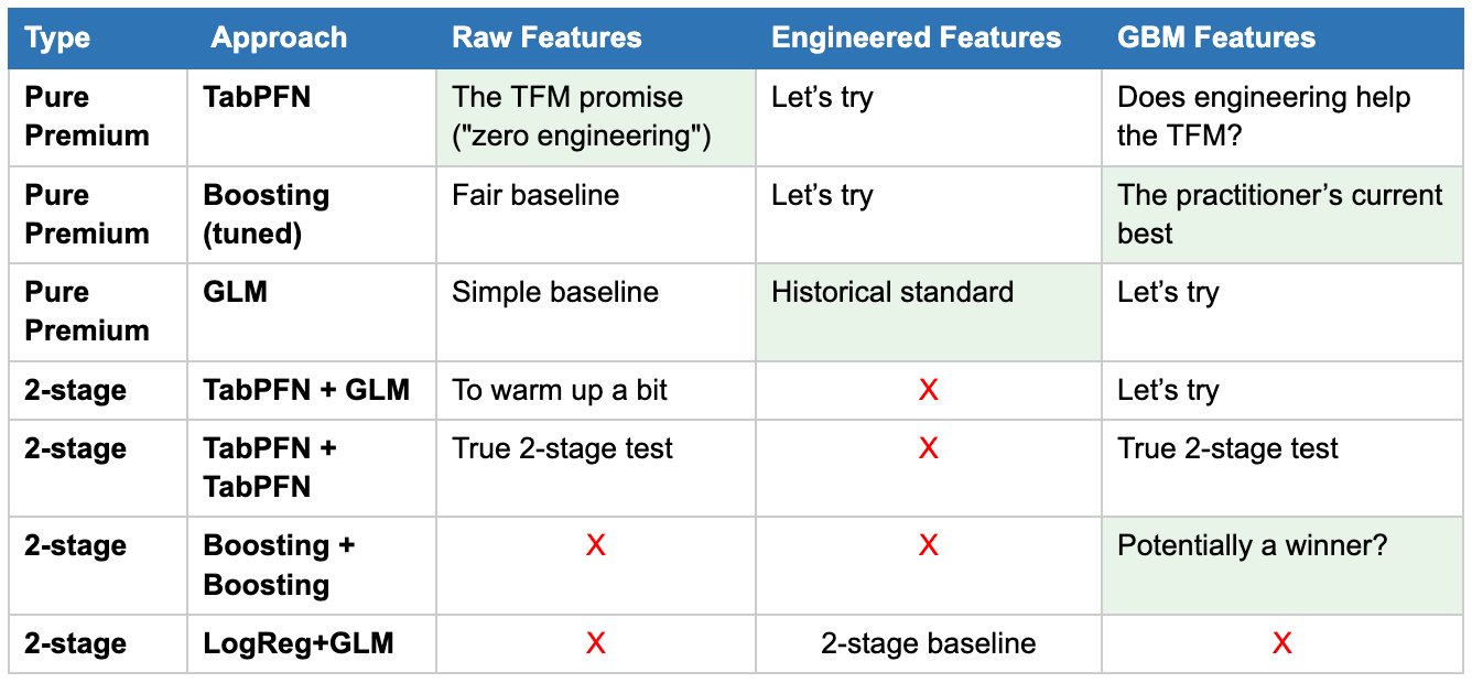
The feature sets. Three of them, each designed to give a different class of model a fair shot.
Raw. Minimum preprocessing. Categoricals (Area, VehBrand, VehGas, Region) converted to ordinal integers. Numerics passed through as-is. This is the TFM promise: “just give me the data.”
GLM-engineered. Actuarial transformations designed for linear models: bonus-malus binning, age bands, vehicle power groupings, log-transformed density, and target-encoded regions. GLMs can’t learn non-linearities on their own, so these features do that work for them. This is what a traditional pricing actuary would have built in 2015.
GBM-engineered. Designed for gradient-boosted trees: no binning (trees handle splits themselves), raw numerics, plus some business-engineered interaction features that tend to help tree models capture structure faster than they’d find it on their own. This is closer to what a modern practitioner running XGBoost in production would use.
The reason for three feature sets rather than two is that “engineered features” is not a single thing. GLM-friendly engineering and GBM-friendly engineering are genuinely different - they serve different modeling assumptions. Testing TabPFN against both keeps the comparison honest.
The full matrix. Combining the modeling approach x feature set x model family gives a grid. Some cells don’t make sense (you don’t run a hurdle GLM on raw features - the whole point of GLM features is to make GLMs work), so I dropped those. What’s left:
The metrics. Five of them, because model rankings flip by metric, and I want you to see that with your own eyes.
Tweedie deviance. The right metric for pure premium. This is what the business cares about.
Poisson deviance. The right metric for the frequency component.
Gini coefficient. Measures how well the model ranks policies, independent of whether the absolute predictions are calibrated. A model with a great Gini but bad Tweedie can still be useful if you’re segmenting customers rather than setting prices.
RMSE and MAE. The generic baselines everyone recognizes. Useful mainly to show that they disagree with the domain metrics.
Training setup. Five-fold cross-validation with out-of-fold predictions. Optuna tuning on a held-out development set with inner 3-fold CV, done once per model family and then locked - I didn’t re-tune per feature set, because that would be an infinite experiment and also not how anyone deploys. Target encoding and any leakage-prone transforms are fit only inside the training portion of each fold.
TabPFN gets a special note: it has a training-size limit that matters in practice. I’ll cover what I did about that in Stage 2, where it becomes relevant.
What I’m not testing. No ensembles, no stacking, no model averaging. The question is “how does a TFM compare to standard practitioner tools,” not “can I win a Kaggle competition by blending everything.” A stacked ensemble of all of these would probably beat any single model, but it wouldn’t tell you anything about the TFM paradigm.
The code and reproducibility notes are in the GitHub repo.
Claim amounts, when they happen, are right-skewed: most are small, a few are catastrophic. This combination - … - is why Tweedie exists as a distribution family
If you worked with insurance pricing, you might have encountered the freMTPL2 dataset, which consists of Frequency and Severity parts. It contains around 680k policies, and there are nine features (driver age, vehicle age, vehicle power, vehicle brand, gas type, region, area code, density, bonus-malus), one exposure column, and the claim outcomes you’re trying to predict - separate in frequency and severity datasets.
If you’ve never seen insurance data before, here’s what makes it structurally different from the tabular datasets you’re used to.
Exposure isn’t a feature. It’s a measurement window. Most policies aren’t observed for a full year - they get written mid-year, canceled, renewed, or switched. A policy observed for three months with one claim is fundamentally different from a policy observed for twelve months with one claim. In GLMs, this is handled elegantly: you pass log(exposure) as an offset term, and the model predicts a rate. In XGBoost and LightGBM, you pass exposure as a sample weight, which is close enough. In TabPFN, you pass it as… well, this is where it gets interesting, and I’ll come back to it.
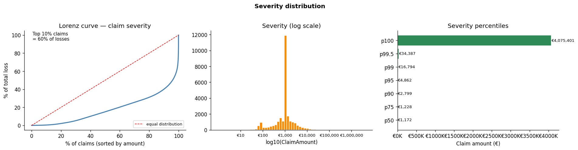
The target is weird. About 95% of policies have no claims at all. Of the 5% that do, 99.8% have exactly one claim - only 0.2% have more than one. Claim amounts, when they happen, are right-skewed: most are small, a few are catastrophic. This combination - a spike at zero and a positively skewed tail - is why Tweedie exists as a distribution family. It’s also why a naive RMSE on this data tells you approximately nothing.
Just so you have a brief idea of what data looks like, here are a couple of charts
Target analysis
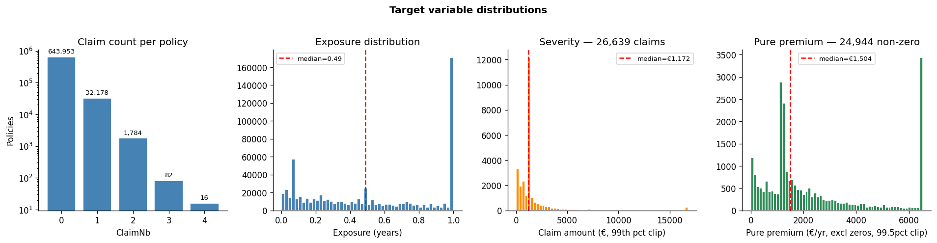
Frequency analysis
Severity analysis
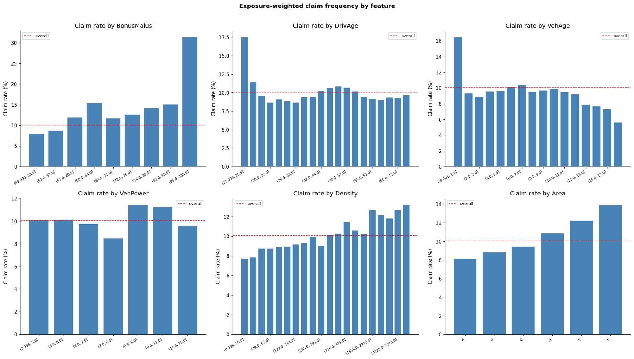
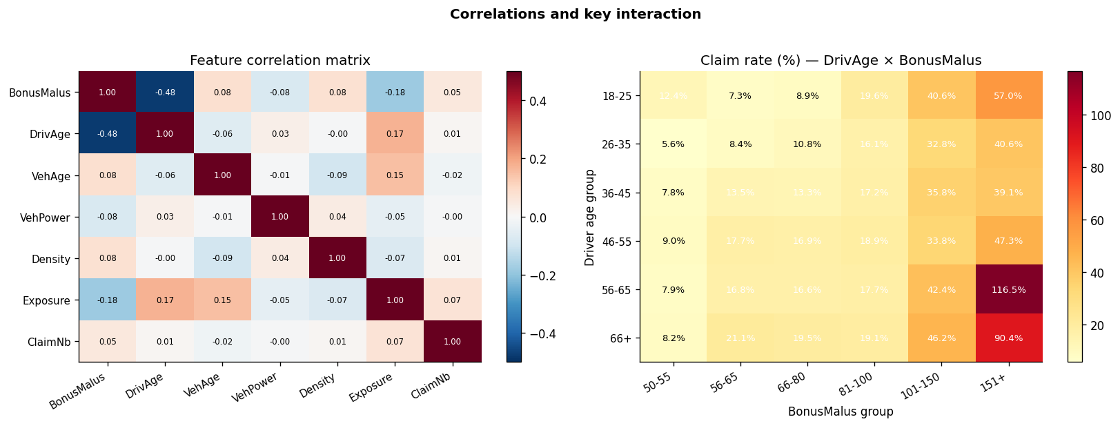
Features Analysis
The exposure question for TabPFN. This is where the TFM paradigm meets insurance reality for the first time, and it’s worth a paragraph.
TabPFN has no offset parameter. It has no sample weight parameter that behaves like GLM weights. It just has: features in, target out. So when you want to predict something exposure-dependent, you have to find a workaround. Mine was - pass exposure as a feature. The model learns to use it, or doesn’t. No guarantee it’ll behave like a proper offset - in fact, almost guaranteed it won’t - but if your target is already a rate (like pure_premium = ClaimAmount / Exposure), this is the correct thing to do. Exposure becomes a contextual feature the model can condition on.
The first time I ran TabPFN on pure premium with the Tweedie metric, every traditional algorithm landed around 90. Raw TabPFN came in at 61,000,000.
For insurance pure premium modeling, we model with Tweedie deviance - a distribution family that interpolates between Poisson (frequency) and Gamma (severity), well-suited to the zero-inflated, right-skewed nature of claims data. This is just an established standard practice for this family of problems.
For GLMs and Boosted Trees, we have Explicit Loss Minimization. The model parameters are updated iteratively so that each step moves in the direction that reduces this specific loss.
TabPFN works entirely differently, as I’ve understood so far. At inference time, you hand it your training set and test set simultaneously; the model reads your training data as context and predicts the test labels in a single forward pass, no gradient updates, no iterative fitting - a paradigm shared by many TFMs, not just TabPFN. The upside is striking - no training loops, tuning, or leakage introduced by incorrect validation. But this also means TabPFN, for example, cannot accept a custom loss function.
This fundamental difference has two practical consequences for pure premium modeling.
1. The calibration problem
The first time I ran TabPFN on pure premium with the Tweedie metric, every traditional algorithm landed around 90. Raw TabPFN came in at 61,000,000. Yes, almost a million times worse. This was my first experiment with TabPFN, at the time using version 2.6. TabPFN3.0 was an improvement - I was re-running my experiments and landed at around 784,500. Not millions, but still a hundred-thousand-magnitude difference.
I stared at this number for longer than I’d like to admit. Was it a bug? Wrong scale? Had I fed the target in euros instead of thousands? I checked. I re-ran. Same number. Consistently, astronomically wrong.
Apparently, it isn’t a bug. It’s structural. TabPFN’s predictions aren’t calibrated to the Tweedie scale. The model ranks policies reasonably well (good Gini) but systematically mis-estimates the absolute level and skewness of the distribution. Tweedie deviance punishes miscalibration brutally, which is exactly why it’s the right metric for pricing - if your absolute predictions are off, your premiums are off, and your P&L is off.
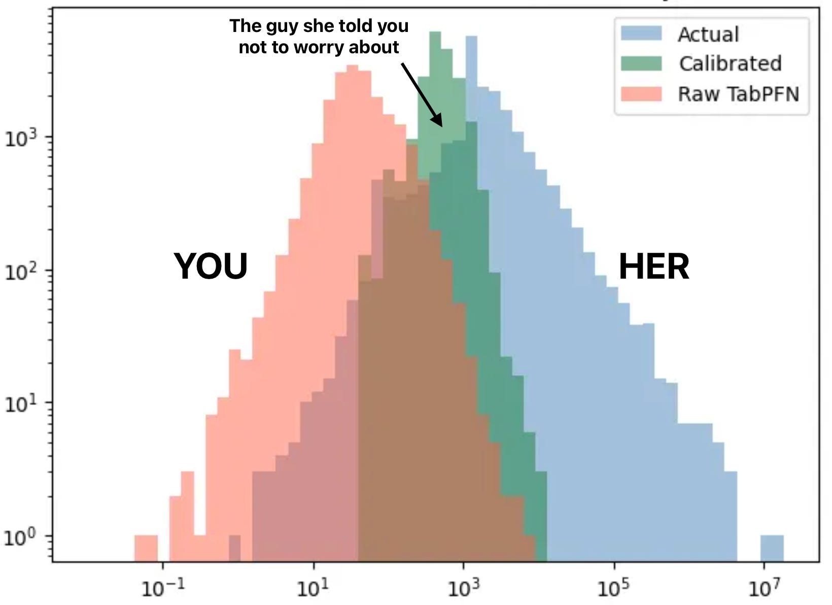
Here’s what this looks like on a log-log plot of predictions vs actuals (for TabPFN 3.0):
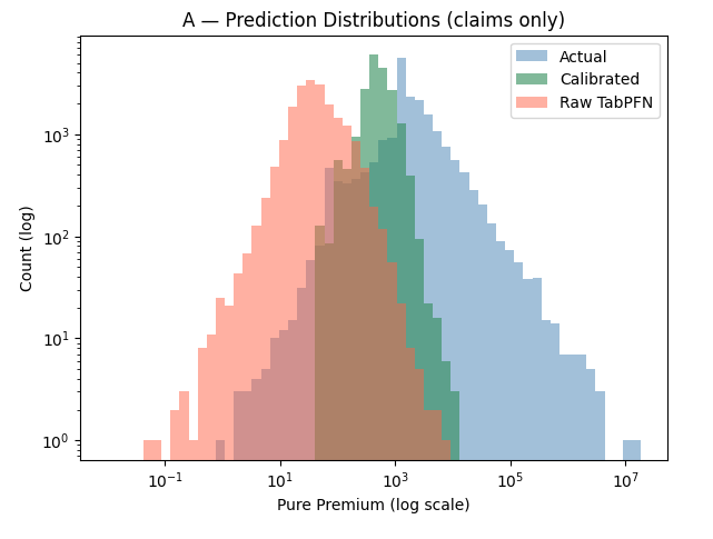
Raw TabPFN (red) is shifted left by roughly an order of magnitude. The bulk of predictions sit in the 1–1000 range, while actual pure premiums center around 100–10,000. That explains the presence of thousands in Tweedie for raw TabPFN in calibrated Tweedie.
To investigate whether this can be solved, a post-hoc recalibration layer - a single-variable Tweedie GLM fitted on out-of-fold predictions - remaps TabPFN’s output into a Tweedie-optimal scale. Whether this recovers meaningful performance is one of the core questions the experiment addresses.
Calibration (green) fixes the location but slightly damages the spread. The recalibrated predictions snap to the right neighborhood - roughly centered where actuals are - but they’re compressed into a narrow band (again, remember it is log-log, I promise you, non-log version is a disaster of a chart, so let’s stick to this one). A single-variable Tweedie GLM remapping can shift the center of mass, but it can’t reconstruct the heavy right tail that actual insurance losses have. Everything gets squeezed toward the mean prediction.
The Gini, by the way, is identical*, confirming our doubts.
* rather, almost identical, depending on the calibration strategy
Going forward, every TabPFN number I report is the calibrated version unless I say otherwise. Raw TabPFN on pure premium is not a serious benchmark.
2. The 10K training limit
If you think I’m done with TabPFN caveats, think twice. TabPFN has a parameter that represents the maximum number of rows for training. I used 10,000 rows mostly because this number directly and heavily impacts prediction time to the point that 50k training rows were very slow even on a good GPU machine (RTX 4090). My experiment of getting 5 CV scores for a 10k limit took 30 minutes, and for a 50k limit, it took 3 full hours (partially because of calibration)
Also, weirdly enough, more training context made the model slightly worse. I still haven’t figured out exactly why. If you have theories, I’d love to hear them. My best guess is that TabPFN’s attention mechanism isn’t equally effective across all training-set sizes, and the sweet spot is domain-dependent. But this is speculation, and I don’t want to pretend otherwise.
What’s not speculation: 670K policies minus a test split is still far more data than TabPFN can ingest in one forward pass. So subsampling is not a nice-to-have - it’s the default. Every TabPFN result you’ll see in the table below uses 10K training rows, subsampled per CV fold. The suffix 10K on model names reflects this.
This is another TFM-class observation, not a TabPFN-specific one. In-context learning scales with context length, and context length scales with memory and compute. Every pure TFM will have some effective training-set ceiling. Where that ceiling sits and how gracefully performance degrades near it will be a practical question for adoption across every data-rich domain, most of which are enterprise domains.
There were many small issues, gotchas, caveats, fixes, and workarounds I will not be explaining, but thanks to Claude Code, I was able to make it work in a reasonable amount of time. Feel free to check them in my GitHub repository (in particular /src folder).
Finally, the juicy part, you were here for, right?
Five-fold CV, out-of-fold predictions, all metrics computed on the same folds. The main findings, in order of “how loud should I say this”:
Rankings flip by metric, and it isn’t subtle. The model that wins on Tweedie is not the same as the one that wins on Gini, nor is it the same as the one that wins on MAE. If you publish a TFM benchmark on a single metric, you are not measuring model quality - you are measuring metric agreement with your chosen setup. This was true before TFMs, but TFMs make it visible in a way that boosting-vs-boosting comparisons didn’t.
Boosting might still be all you need. LightGBM-gbm ranks first on Tweedie, first on Poisson, and respectable on other metrics. The honest practitioner takeaway: for structured insurance pricing, a well-tuned boosted tree with GBM-friendly features is extremely hard to beat in a fair head-to-head matchup.
TabPFN in hurdle mode is super competitive - when configured right. TabPFN_hurdle_full_raw ranks third on Tweedie/Poisson, first on Gini/RMSE, and has the highest average rank on the leaderboard. This is the most favorable configuration for a TFM on this problem: decompose the zero-inflated target into a classification step and a severity step, then let TabPFN handle each piece separately.
TabPFN in pure premium mode barely beats the simplest baseline. TabPFN_10K_raw, TabPFN_10K_engineered, and TabPFN_10K_gbm sit near the bottom of the ranking table, roughly level with plain Tweedie GLM. After everything - calibration, subsampling, feature engineering - the pure-premium TabPFN is not competitive with a tuned LightGBM.
Raw, uncalibrated TabPFN wins on MAE and loses to Tweedie by a factor of 90,000. This is the single clearest illustration of the rankings-flip-by-metric finding anywhere in the table. It’s also a warning about what “best on MAE” actually means when MAE is not the metric your business is paying for.
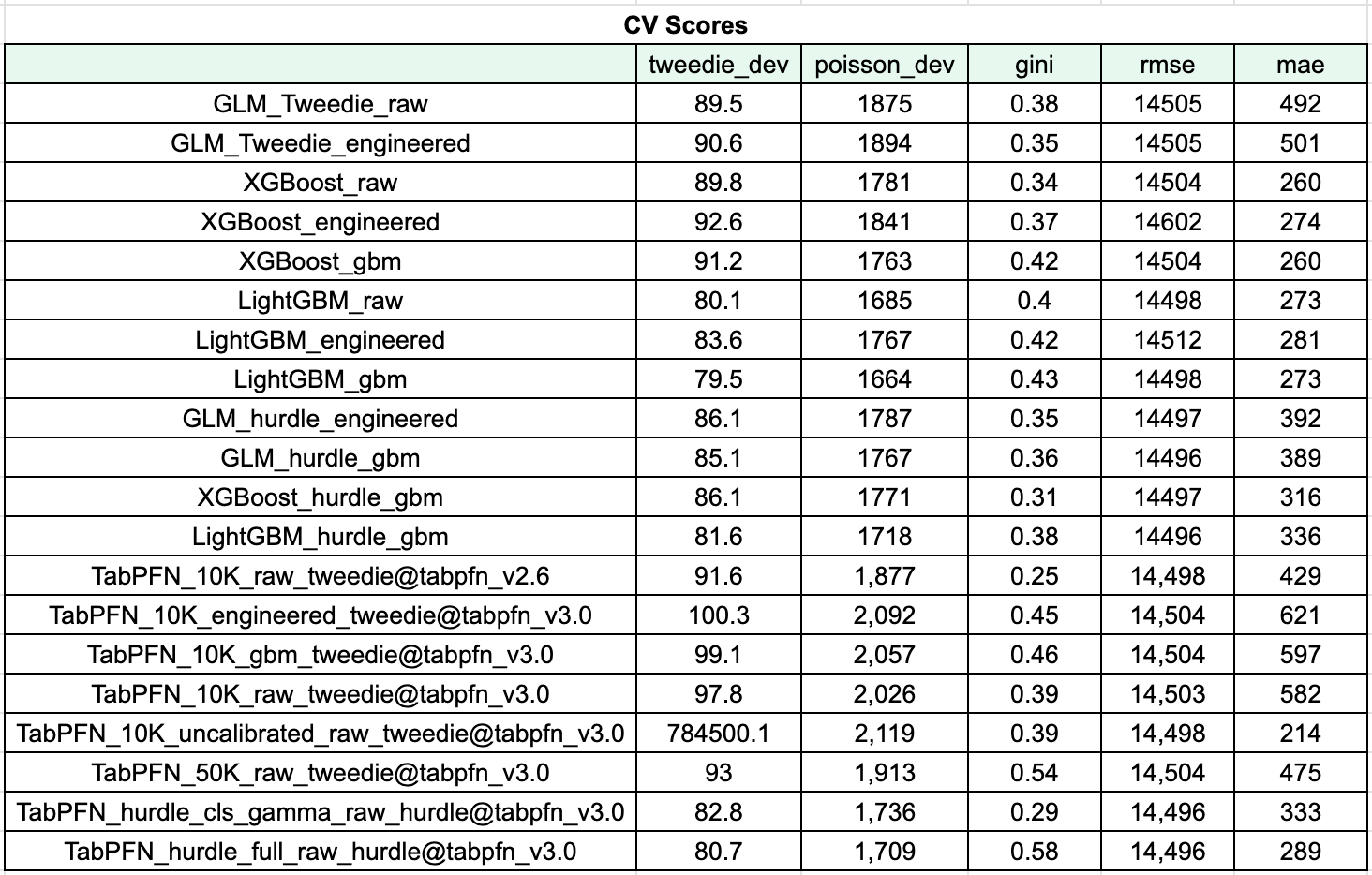
_raw, _engineered, or _gbm suffix relates to the type of feature engineering we did.
More specifically, you can see how models are different in the next metrics ranks table:
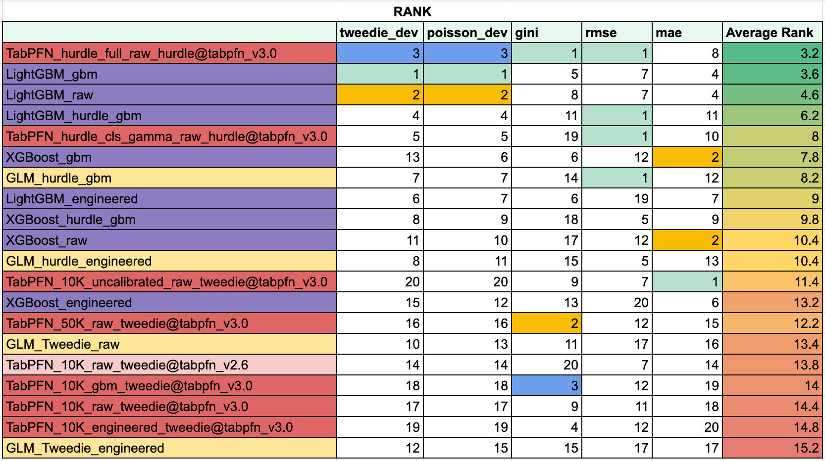
About “hurdle” - a quick technical note. This is the two-stage approach I flagged in experiment design: classify whether a claim happens, then predict severity given a claim. For TabPFN, I tested two flavors: hurdle_full uses TabPFN for both the classification step and the severity regression, while hurdle_cls_gamma uses a GLM for classification (it’s a 670K-row binary problem, which is above TabPFN’s comfort zone) and TabPFN for severity only.
A few more observations worth flagging before we move on.
The feature-engineering gap is smaller than I expected. TabPFN_10K_gbm (tree-friendly engineered features) and TabPFN_10K_raw (raw features) are close on most metrics, and TabPFN_10K_engineered (GLM-friendly features) actually does slightly worse than both. This roughly confirms the TFM’s promise in engineering: you don’t need to hand-craft features for the TFM the way you do for a GLM. But it does not confirm the stronger version of the claim, which would be that TabPFN with no engineering beats Boosting with full engineering. That isn’t what happened here.
GLM Tweedie models - both raw and engineered - are near the bottom. Maybe that’s partly a freMTPL2 property and partly a consequence of comparing Tweedie deviance between a model fitted with a Tweedie loss and one fitted to rank policies well. Either way, the industry-standard GLM is easy to beat with modern tools, and the hurdle GLM is notably more competitive than the pure-premium GLM. That, too, is a finding.
Versions instability. Can I humor you one more time? The same config for the 2.6 model version has a much worse Gini (rank 20), but new generation models perform worse on RMSE/MAE. I even calculated the Pearson correlation between the 2.6 and 3.0 predictions: 0.27. This is what you need to know about the version stability of these models. One day you wake up, accidentally upgrade the library, and … Well, let’s say if you like to work night shifts and weekends - this one is for you.
I was disappointed by one thing specifically. The calibration step - building a post-hoc GLM wrapper just to make TabPFN’s scale usable - required tricky, careful out-of-fold management that I didn’t think I’d be doing in 2026. If a TFM is being pitched as the “no feature engineering needed” future, shipping a calibration layer with the library seems like the next obvious step. Right now, you build it yourself.
So this is it on the metrics. But on-paper rankings are one thing. What happens when these models actually price policies against each other? That’s Stage 3.
TabPFN wrote 100% of the book against every competitor - and lost all money doing it.
I want to start with the business value translation, as it feels natural after discussing metrics. Because a better pricing model is not the one that is better in Tweedie, Gini, or any other artificial metric - it is the one that improves the portfolio economics. Besides that, a new pricing model can create value in many other ways
Better customer mix after price changes
Better competitiveness in specifically attractive customer segments
Simpler and more stable rules to reduce operational friction
Of course, we are not going to do a deep dive into this, but we merely want to understand how best on-paper models translate into business value.
The wrong approach here would be for each model to sum up all the premiums, subtract all the losses and give this number to CFO (I’ve seen people actually doing this) - as this just favors models that overprice. But this doesn’t win you business.
The cleanest approach (or family of approaches) is champion-challenger rotation: each pricing model receives a policy, writes it, and inherits its associated losses. The policy assignment can be randomized, but personally, I am not a fan of it - a handful of catastrophic claims can swing the whole result based on which model got unlucky. So I used a variant that’s closer to what actually happens in a competitive insurance market: an auction.
The rules are simple. For each policy in the holdout set, every model produces a price. The lowest-priced policy wins and inherits any claims it generated. We tally up premiums collected minus losses incurred, and we see who made money.
With Tweedie, every model gets graded on every policy. In an auction, models only get graded on the policies they actually chose to underprice - which is exactly how insurance companies experience their pricing models in the wild. A model that’s great on average but systematically cheap on bad risks will win lots of business and lose money on all of it. That’s called adverse selection, and it’s how insurance companies go bankrupt.
I ran head-to-head auctions between a curated selection of approaches. Each cell in the matrix below shows the results of a two-model auction: the percentage of the book each model won and the net profit (premiums collected minus claims paid) each generated on the policies it wrote.
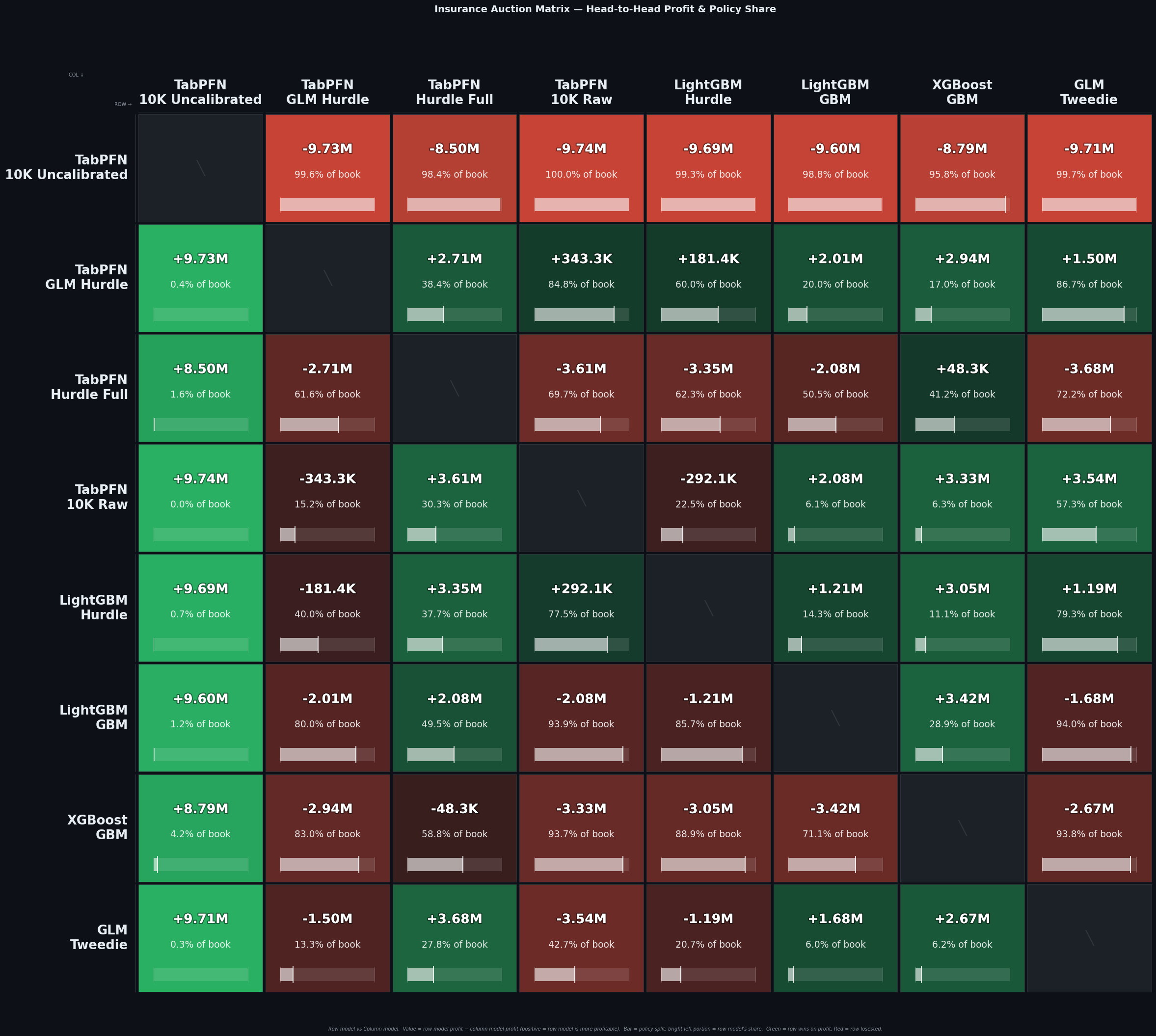
A few things jump out immediately.
TabPFN-uncalibrated (row 1) wrote 100% of the book against every competitor- and lost all money doing it. This is the single most important finding in Stage 3, and it’s one you cannot see in any of the Stage 2 tables. Uncalibrated TabPFN in pure-premium mode systematically underprices across the entire portfolio. It’s not that it’s wrong on a few segments; it’s that it’s cheaper than every other model on every segment, so it “wins” every auction and inherits every loss. In production, this would be a bankruptcy machine.
But! Calibrated TabPFN (a.k.a “the guys she told you not to worry about”, row 4) was actually quite good. I was really surprised to see it there, considering the metrics table, but here we are. It is the best single-stage model in the auction, losing only to hurdle approaches. What is awesome is that in most cases, it writes less than a third of the business, potentially correctly identifying high claims policies with a high degree of confidence.
TabPFN hurdle with GLM was the close winner, winning only $200K from LightGBM-hurdle-gbm in a head-to-head. The model was #5 in the metrics table, so this is another example of how potentially misleading benchmarking can be. This is the most credible TFM result in the entire post: in a structurally favorable configuration (hurdle mode, tree-friendly features, the full two-stage TabPFN pipeline), the TFM is genuinely competitive with the best traditional approach. On a problem where traditional tools have had thirty years of refinement.
The top-ranked models on Tweedie did not win the auction. The auction picture doesn’t show all of the models in the auction results - it shows the top models from the metrics table alongside some interesting findings. Those are still better than the ones left over, so the perception that those models are bad overall is wrong. There are just some slightly better. A mediocre model that refuses to be catastrophically wrong can be more profitable than a sharp model that occasionally is.
What this tells us about TFMs specifically.
And despite the fact that I consider this a win for TFMs, and TabPFN in particular, the win didn’t feel like winning. It felt more like swimming against the current until it finally let up. Like a gold miner panning sand all day and finding a nugget the size of a fingernail - nothing to write home about. But a win is a win.
Three things, in increasing order of importance.
First, for insurance pricing, TFMs in pure-premium mode are not deployable without substantial wrapping. The calibration issue from Stage 2 translates directly into adverse selection in a competitive market. If you ship uncalibrated TabPFN as a pricing model, you will underprice bad risks and lose money. What could happen if you have no industrial experience and just decided to deploy it because it is best on MAE?
Second, TabPFN in hurdle mode closes the gap. Decomposing the problem into “does a claim happen” and “how bad is it given a claim” plays to the TabPFN’s strengths - classification and well-behaved regression - while sidestepping the pure-premium calibration trap. The best TabPFN configuration is roughly 50/50 against the best Boosting configuration. Nevertheless, I consider this a win. A natural question is: could we achieve better classification with GBMs than with GLMs, and improve it further? Maybe! You can do this test as well. And despite the fact that I consider this a win for TFMs, and TabPFN in particular, the win didn't feel like winning. It felt more like swimming against the current until it finally let up. Like a gold miner panning sand all day and finding a nugget the size of a fingernail - nothing to write home about. But a win is a win.
Third - and this is the one I want to underline - the auction finding does not show up in any standard TFM benchmark. Maybe they should not, but a Tweedie deviance table would have told you that the calibrated pure-premium TabPFN is mid-pack. An auction tells you - it is actually not bad. The gap between those two verdicts is what “can TFMs survive the real world” actually means in insurance. And I’d bet real money that this gap shows up in other regulated, high-stakes domains too - credit pricing, reinsurance, healthcare risk adjustment. Anywhere the business decision is “do I write this policy, yes or no, at what price,” the on-paper metric will understate the deployment risk.
Kudos to Prior Labs, by the way, for extensively documented interpretability examples. You can take a look, and you will see partial dependence, feature selection, and individual SHAP waterfalls that will warm your heart, like a data center with GPU clusters generating AI videos of cats playing drums, warming the atmosphere.
Insurance is not one of those domains where “trust me, bro” is a sound strategy. Interpretability here is not a nice add-on on conference slides - it is a part of the product. Interpretability of your pricing model is a distinction between the auditor taking you to lunch and you taking them to lunch, but they refuse to even see eye to eye with you. This was the reason why boosting algorithms, while superior to traditional GLMs, did not win the hearts and minds of regulators at first. Until we have seen SHAP importances or permutation-based tree feature importances. And then it took 5 years to explain this to your regulators.
I want to test whether interpretability is practically usable, not just theoretically possible. Can I get explanations that are stable, legible, and decision-relevant? Can I compare them to mature alternatives like TreeSHAP without creating a new framework around model behavior?
If you saw my expectations in Post 1, you might remember that I did not expect much, and you know what? I was right! I could have just left you this article by Christof Molnar to read and be done with it. But I wanted more.
The TabPFN authors claim to support various interpretability techniques, so I decided to try them. But I thought I would try KernelSHAP first
KernelSHAP (50 rows): 11143.6s (185.7 min)
Slowdown vs TreeSHAP: 121632× times slower
Wow, 3 hours to get 50 samples. TreeSHAP for boosting algorithms was just 120,000 times faster. I know what you think: “Hey, I can leave the code running those importances and claim to my boss I was working” (while actually doomscrolling). That is apparently the only positive I can find.
You cannot perform any analysis with this level of latency, but this should set expectations for the potential latency of the interpretability code for TFMs in general. That is where I decided to look into TabPFN’s interpretability documentation.
Their docs point to tabpfn_extensions.interpretability, built on top of Shapiq. The pitch is actually clever: instead of KernelSHAP’s trick of marginalizing features by filling them with random samples from a background set (and then asking the model to score rows it has never seen in its life), the TabPFN explainer removes features by re-contextualizing the Bayesian in-context learning. So the explanations are faithful to how the model actually reasons, not to how a generic black-box approximator imagines it reasons. In theory, this is the cleanest SHAP story going.
Native Shapiq (50 rows, budget*=64, 500-row context, RTX 4090): 5,988s (~120 min), 119s/row.
So, roughly 1.5× faster than KernelSHAP. Which is a real improvement - and still about way slower than TreeSHAP on Boosting for the same 50 rows. The doomscrolling window shrinks from “half a working day” to “long lunch plus coffee”, but you are still not running this in any pricing workflow with a feedback loop shorter than a week. Also, see the “budget” in there?
* Quick crash course. What is this budget thing in Shapiq? SHAP in nature is 2^x in complexity, since you need to see the average change in prediction when you add each feature to every possible subset of the other features, and all possible subsets of the set with X members is 2^x. If you have 9 features, 2^9 is 512. This is your default budget. By decreasing the budget, you can discard some subsets and get a SHAP approximation.
Feature importance, for what it is worth, looks sensible, or as Mira Murati would say “directionally right” (as it could be on a 50-row sample):
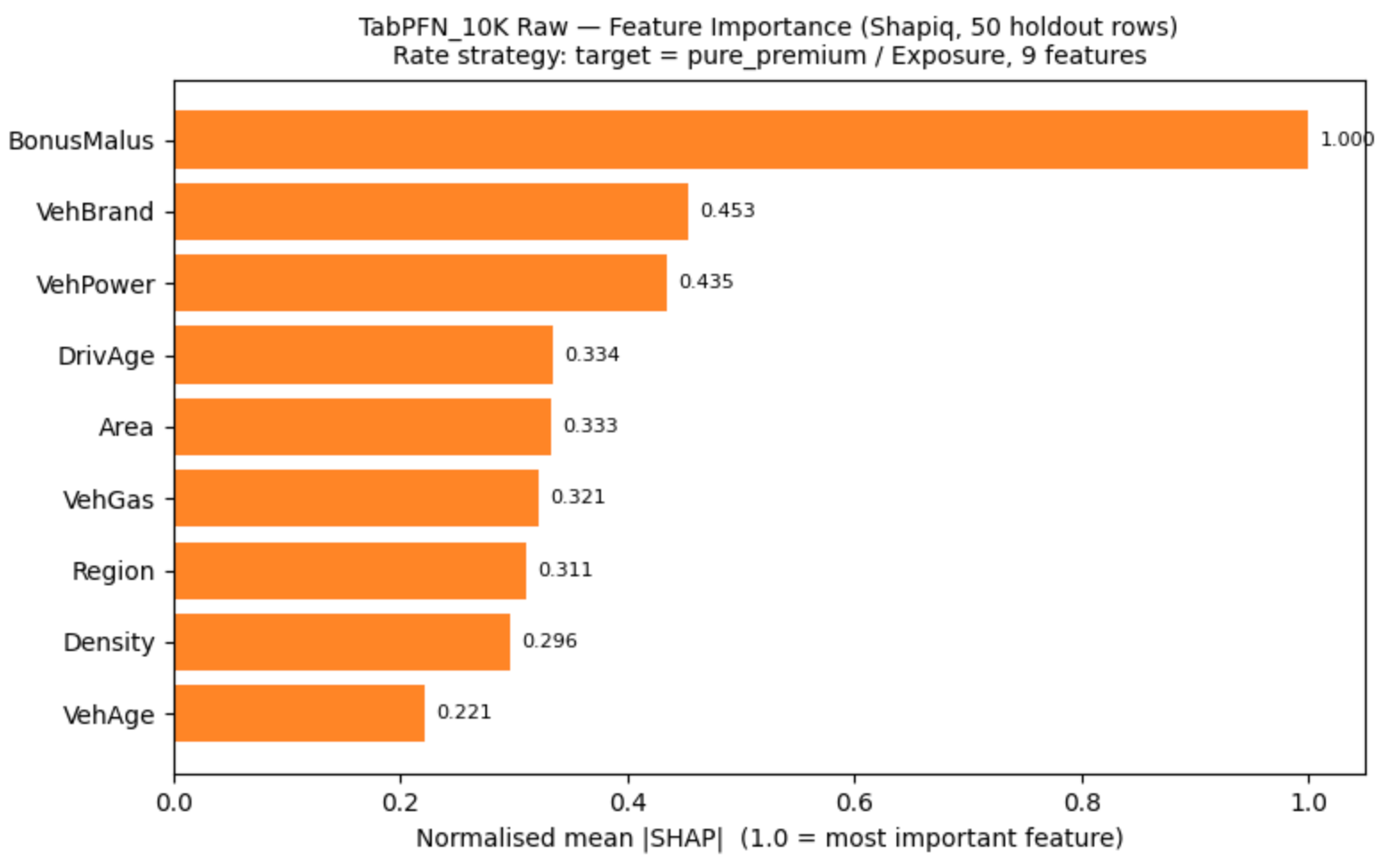
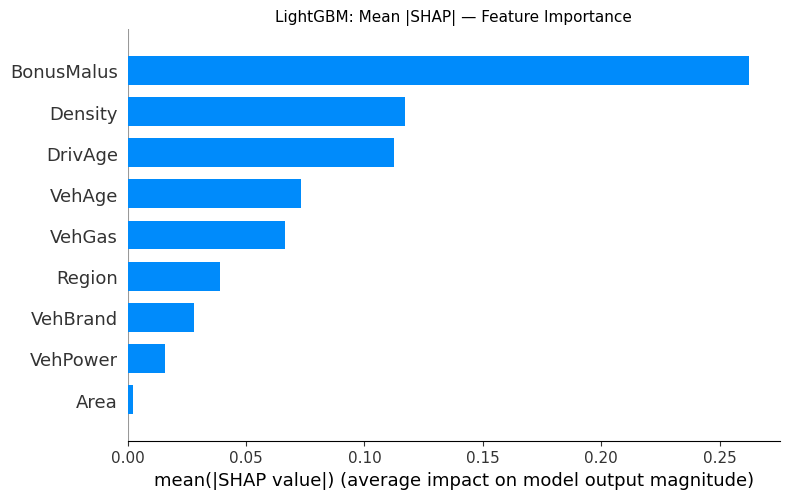
For example, LightGBM feature importance looks similar but not exactly.
Kudos to Prior Labs, by the way, for extensively documented interpretability examples. You can take a look and see partial dependence, feature selection, and individual SHAP waterfalls that will warm your heart, like a data center with GPU clusters generating AI videos of cats playing drums, warming the atmosphere.
But even here, I could not get through. I tried their feature_selection helper, which is supposed to identify the minimal feature subset that preserves performance. It picked {VehBrand, VehGas, VehAge, DrivAge, BonusMalus} in 214s - reasonable, except the follow-up evaluation step died with a CUDA OOM while calling .predict() on the 135K-row holdout. The error message itself helpfully suggests you batch your predictions manually. Which is fine advice, except the helper that produced this message is the helper whose whole job is to wrap this step for you. You get a “hey, handle your own batching” from the library that sold you on not handling your own anything.
So, the summary of practical interpretability is that your options are very limited. They are so limited that, beyond something simple (PDP, permutation, ALE etc) on small batches of data, everything else is unusable. Interpretability should be fast and trustworthy. If you want to use this in front of an auditor, you can - once. You will not enjoy the second time. And it is not only about auditors, in general whenever I try to debug the model, I always go for feature importances and PDPs. GPU requirement for this does not sit with me well.
TabPFN actually has some advantages compared to others - it has a distillation engine (a tree-based approximation), but it’s only available in the Enterprise edition.
It is quite often overlooked how exactly models work in production. But not here - here we cover all the necessary aspects of the ML project lifecycle, like inference, for example. I benchmarked inference the boring way: predict 10,000 holdout rows across 5 runs, then take the median latency. Hardware: RTX 4090, 16 vCPU, 62 GB RAM.
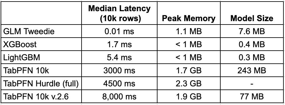
XGBoost and LightGBM ship as compact artifacts and score quickly. TabPFN is an in-context learner. At inference time, it loads the model weights (~100-400 MB for the transformer) plus the entire training reference set into GPU memory, then runs attention between your query rows and the reference rows. So the 1.7 GB is roughly: model weights + 10K reference rows encoded as tensors + attention activations + output buffers. Scale the reference set and query batch size up, and this grows. (Readers who know the architecture better than I do, flag anything I’ve gotten wrong)
In a typical insurance company’s serving stack, pricing models run on CPU-only containers - think ECS Fargate tasks, Kubernetes pods on c-family instances, maybe a simple Flask app behind a load balancer. The deployment looks like this: pull a 0.3 MB LightGBM artifact from S3, load it, and serve predictions using a few hundred MB of RAM in total. You can run 10-20 model instances on a single 8 GB machine and autoscale at low cost.
But with TabPFN, it is different. First - GPU requirement. These cost 3-10× as much per hour as CPU instances, have longer cold-start times, and most insurance platform teams don’t have GPU-serving infrastructure at all. Autoscaling gets expensive. CPU containers scale to zero when idle and spin up in seconds. GPU containers take 30-60 seconds to start.
Second - concurrency. A 4090 has 24 GB VRAM. At 1.7 GB per inference call, you can run maybe 6-12 concurrent requests before you’re out of memory. My expertise ends here, but you’ll need aggressive queuing or multiple GPUs for true real-time quoting.
And there is latency. The difference is not critical at first glance, but it can be critical depending on how the model is used. If you use it for offline batch scoring (nightly re-pricing, portfolio analysis), then these 8 seconds are manageable. The whole book will run in less than an hour. But for real-time quoting, this is just dead on arrival. Quotes arrive one by one, not in 10k batches, but there is still an overhead cost you will pay. Probably no-go for API-based quoting.
I suspect this situation will be common for all TFMs. To be fair, TabPFN actually has some advantages compared to others - it has a distillation engine (a tree-based approximation), but it’s only available in the Enterprise edition. In the end, assuming distillation preserves accuracy, this is not a problem. But not all TFMs offer such a thing.
Also see - comparing to the 2.6 version, 3.0 has improved the latency by half, which is great. By tripling the model footprint, which is not that great
As I mentioned in the disclaimer, I see TabPFN and other TFMs as an exciting technology. I wanted to believe that this is a hammer for people who were using a screwdriver to hammer nails, or at least a better screwdriver. What I learned is that insurance might still be months or even years away from adopting this technology, despite things are moving very fast here.
But at the same time, I couldn’t help but wonder: if this result is achievable with open-source models, what is possible with enterprise versions? I can foresee Prior Labs having a lot better model that not only saw synthetic data but also insurance data to learn from. Maybe training without a specific metric in mind would still work and yield good results? What if their distillation preserves accuracy, making the deployment process identical to the current one with boosting algorithms? Can we run interpretability experiments better and faster? There is a lot of potential here.
In my Post 1, I asked several questions, and I want to give my honest, brief answers to those. The answers will be based on my TabPFN experience extrapolated to other TFMs.
You actually can. Some features helped a bit, and in the end, you might still want to do some engineering to capture additional signal, but TFMs can capture the signal directly from the raw data. My problem is - you will never know what feature engineering you could do to improve the model - just blindly test and see if it works. But in any case, no engineering is still doing well. So the promise was delivered.
You are not flexible. TFMs tell you the rules to play, and you play along. Custom metrics are a problem. You hack around them. You often don’t know what the TFM actually optimized during training. In my experiment, TabPFN was close to the top on some metrics and dead last on others.
TabPFN has some explainability capabilities, but it cannot scale on demand. Other TFM models may face similar issues - and they will be very slow. I was terrified by the 3-minute-per-row KernelSHAP run to the point that I actually wanted to drop interpretability from the experiment altogether. For example, if I ever run a Time Series experiment, I will not be focusing on interpretability at all.
I don’t see TFM as a basis for a high-load system in the near future. For batch prediction - yes. Distillation that preserves accuracy would flip this verdict. I’ll be watching.