Quick Summary
This is the final phase of solving DLPs. Our goal is to convert a big integer into a product of small prime numbers over our factor base.
We assume familiarity with index calculus techniques. This is part of our series on Practical Index Calculus for Computer Programmers.
Part 1: Discrete Logarithms and the Index Calculus Solution.
Part 2: Solving Pell Equations with Index Calculus and Algebraic Numbers.
Part 3: Solving Index Calculus Equations over Integers and Finite Fields.
Part 4.1 : Pollard Kangaroo when Index Calculus Fails.
Part 4.2 : Pohlig-Hellman Attack.
Part 5 : Smart Attack on Anomalous Curves.
Part 6: Hacking Dormant Bitcoin Wallets in C.
Part 7.1: Gaussian Integers Introduction.
Part 7.2: Linear Algebra Phase.
Part 7.3 (we are here): Reduction and Descent by Sieving.
As usual, the code is available on GitHub.
We shall use our database of primes (and their virtual logarithms) from Part 7.2 to solve individual DLPs. We do this finding a factorization of our target into primes over our factorbase. This phase of solving DLP’s is either called the Reduction Phase or the Descent Phase in different books.
Our primary source is (Weber, 1997)1.
We summarize below the steps of the reduction phase.
Find rational reconstruction of target modulo prime.
Find prime factorization of numerator and denominator.
Find appropriate sieving polynomials for each large prime factor (t) modulo prime.
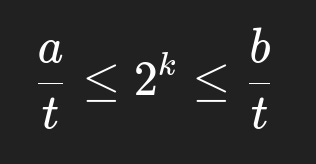
Find k, an exponent of 2 that places t in the range √p/2 ≤ t ≤ √p or equivalently:

Finding k Find the new value of t by multiplying by 2^k.
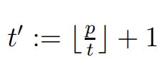
Find t’ such that:

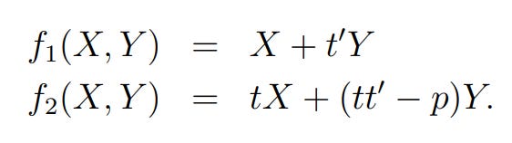
Finding t prime from the modified t Construct sieving polynomials of the form:

Sieving polynomials using t, t’ and p Find each sieving polynomial’s root modulo every prime in the factor base. These are the positions likely to be prime.
Finding a root is setting the lhs to 0. So taking the example from page 28:

Sieve polynomial example from page 28 So the first function’s root look likes:

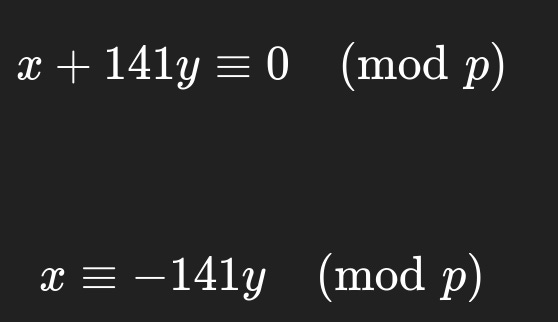
Finding root of f1 This tells us that our desired sieve positions are defined by the formula
x = (-141*y mod p) + k*p
Start sieving
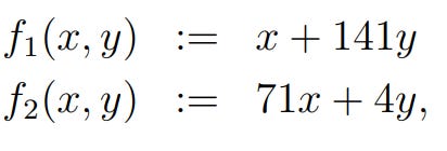
We provide an easy-to-follow example for maximum clarity.
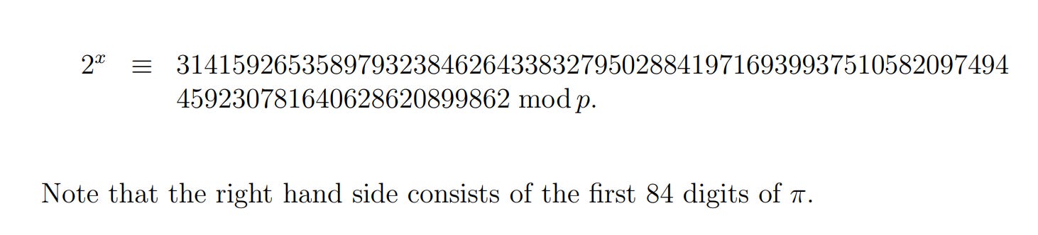
We aim to solve the DLP above where p is the 281 bit prime:
p = 3108193808041961141219111205196826101966010119640309197118051941271219700607191207059We are provided a solution for x and can test in Python:
x = 756823288306878728158503093002882408211087576743681636958030065477607481720402869192
p = 3108193808041961141219111205196826101966010119640309197118051941271219700607191207059

target = 314159265358979323846264338327950288419716939937510582097494459230781640628620899862
res = pow(2,x,p)
assert(target == res)
print(res)
Step 1: Rational Reconstruction
We use FLINT’s fmpq_reconstruct_fmpz function to find a/b:
int reconstructionSuccess = fmpq_reconstruct_fmpz(rationalReconstruction, target, prime);We get this fraction modulo p:

Factorizing the numerator and denominator yields the fraction:

Step 2: Sieving Polynomials
The numerator features the 131-bit number:
p_40 = 2594639391675138810059337116552519320289The logarithm to base 2 of p_40 is ~130.931 bits and we need it in the range 139.339 <= t <=140.339. So we multiply by 2^9.
Now we can construct our sieving polynomials of degree 1 using these constants:
multiplier: 2 ^ 9
t:1328455368537671070750380603674889891987968
tPrime:2339705105383690535824858983784817122332986
t_tprime_minp:66546339222252639135837499089354410305389
Step 3: Sieving Step
We found our sieving polynomial constants. Now we:
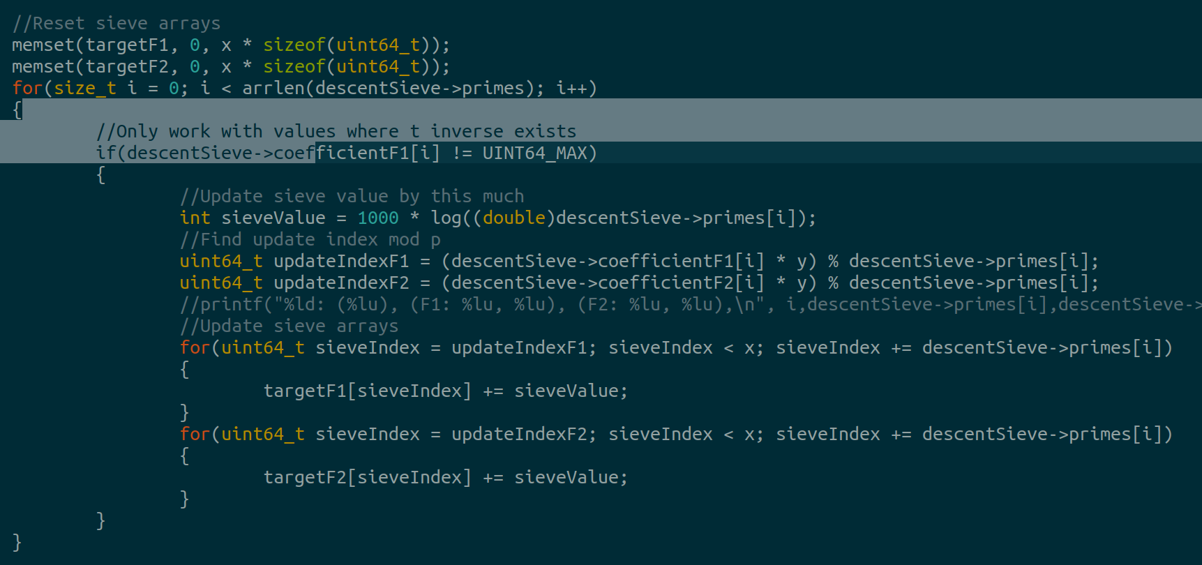
Initialize two arrays for f1 and f2 to hold our sieve logarithms.
Find sieve polynomial roots for f1 and f2 modulo each prime.
Increment by the log of each prime at the root indices.

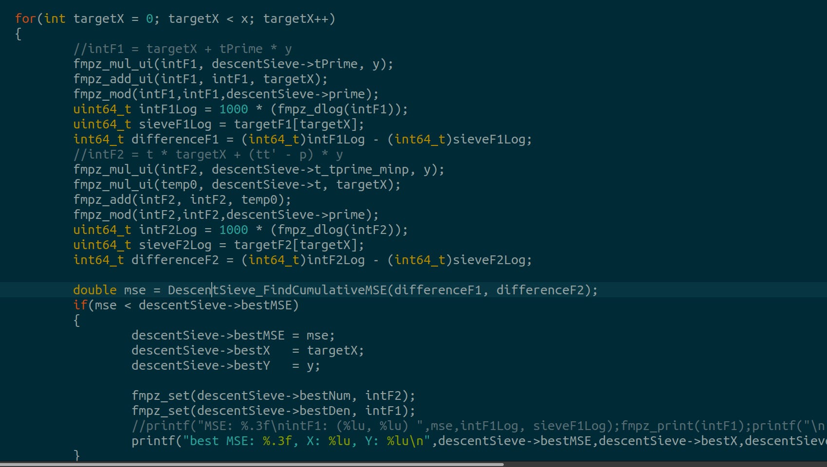
First three sieving steps After the increment stage, the final step is finding out which array elements are closest to our target log. We compare the value of the array to the expected log(F(x,y)) and use MSE.

Using Mean Square Error to find the best sieve indices
Step 4: Sieving Results
Our goal was to reduce the 277 bit target into smaller numbers.
target = 314159265358979323846264338327950288419716939937510582097494459230781640628620899862I ran the sieve for twenty minutes with these parameters:
int factorBaseBitLength = 25 //all primes upto 25 bits
uint64_t sieveX = 30000; //Max x value for sieve
uint64_t sieveY = 1; //Starting index when searching for y
uint64_t maxYoffset = 10000;//Max y value to investigate
and found the representation:

Num: -1107911020245284271895336948767925749763403
(|1| -1 ^ 1), (|3| 7 ^ 1), (|6| 61 ^ 1), (|10| 541 ^ 1), (|14| 15391 ^ 1), (|17| 65677 ^ 1), (|19| 443273 ^ 1), (|20| 619819 ^ 1), (|20| 1012597 ^ 1), (|22| 3438763 ^ 1), (|32| 3620493601 ^ 1), (|2| 2 ^ 105), (|4| 13 ^ 1), (|5| 19 ^ 1), (|14| 12421 ^ 1), (|15| 29833 ^ 1), (|16| 63493 ^ 1), (|21| 2076973 ^ 1), (|23| 5435147 ^ 1), (|23| 6805181 ^ 1), (|34| 12015623357 ^ 1),
Den: 247677069126825671745394690976496808367918
(|2| 2 ^ 10), (|2| 3 ^ 1), (|6| 37 ^ 1), (|7| 79 ^ 1), (|8| 193 ^ 1), (|11| 1103 ^ 1), (|13| 5387 ^ 1), (|14| 9349 ^ 1), (|22| 2691587 ^ 1), (|22| 2804257 ^ 1), (|23| 6069311 ^ 1), (|30| 573129719 ^ 1), (|4| 11 ^ 1), (|4| 13 ^ 1), (|6| 59 ^ 1), (|11| 1129 ^ 1), (|11| 1627 ^ 1), (|12| 2207 ^ 1), (|12| 3779 ^ 1), (|13| 7013 ^ 1), (|16| 64303 ^ 1), (|17| 82997 ^ 1), (|22| 4169521 ^ 1), (|23| 5053313 ^ 1), (|24| 12464909 ^ 1), (|26| 38665007 ^ 1), (|27| 78959357 ^ 1), (|34| 13717458731 ^ 1),
ta
We successsfully reduced our 277 bit target to a product of numbers upto 33 bits lol.
*Running the sieve longer finds better representations
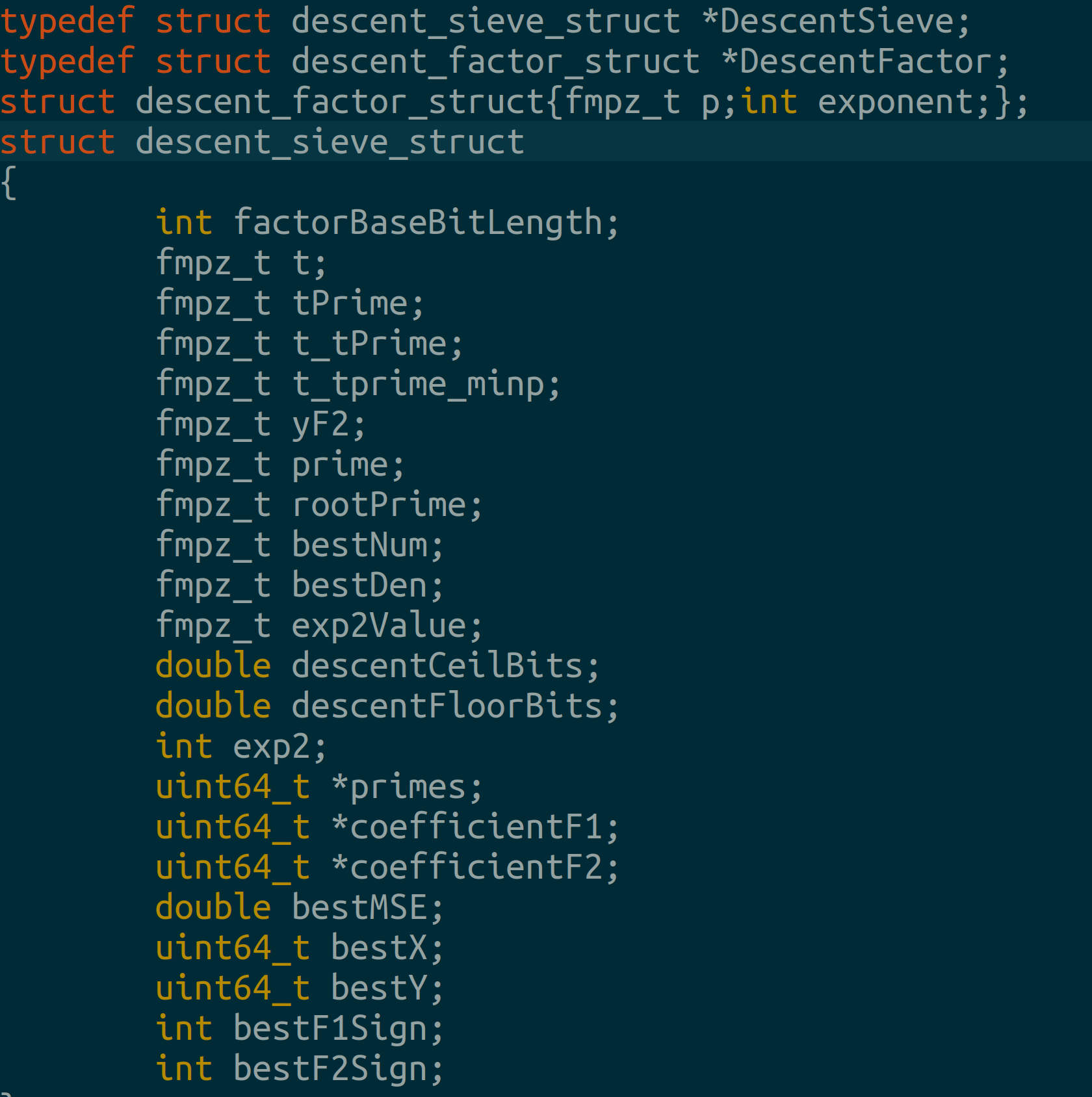
First, we define a data structure to hold our descent variables as defined in (Weber, 1997):
Next, we write a function to find sieve coefficients for each individual prime factor:


Then we write a sieving algorithm:


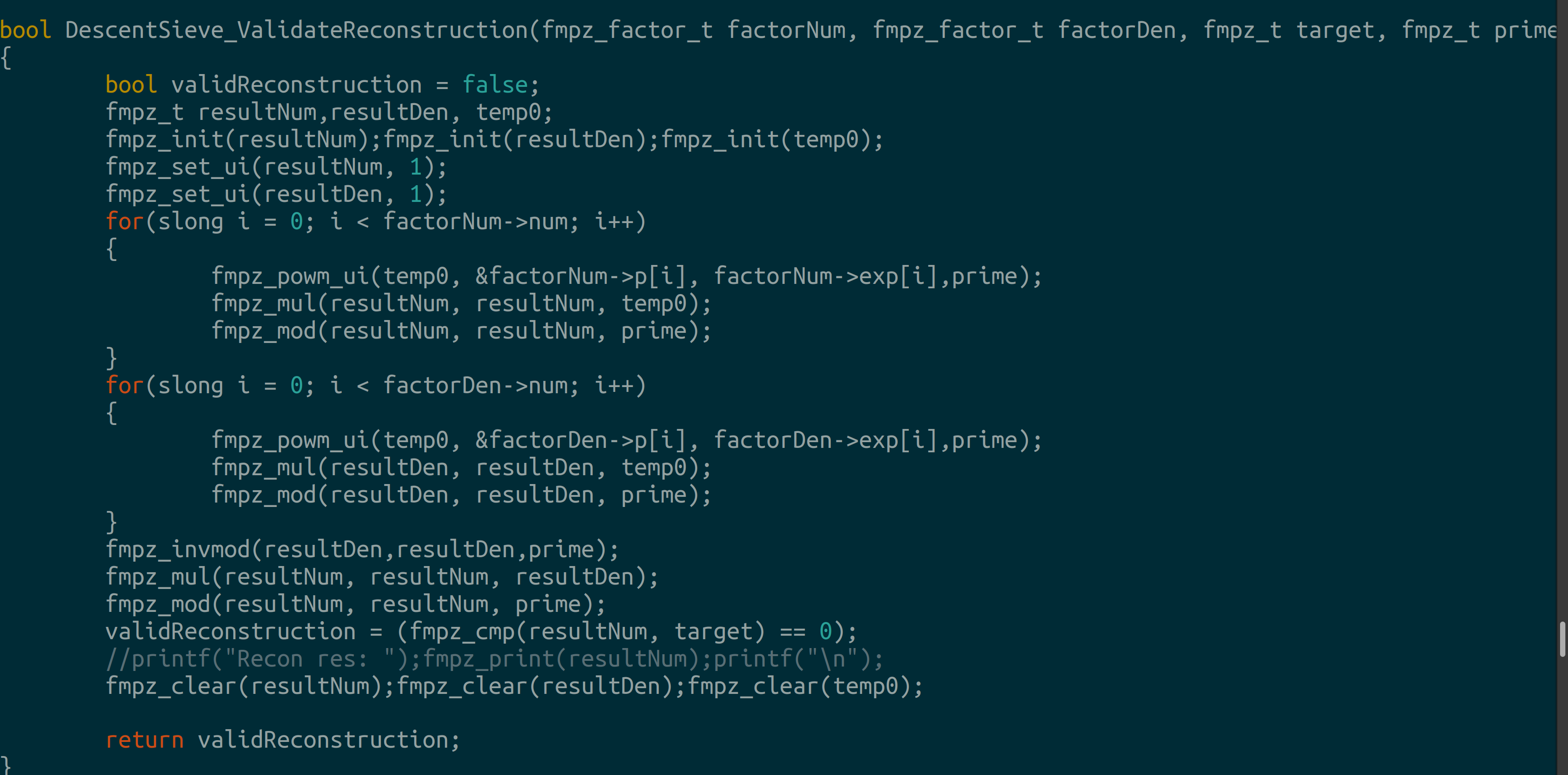
We also write a validator (for our own sanity):
Finally, we write a function to tie everything together:


We run our sieve on the numerical example from before:

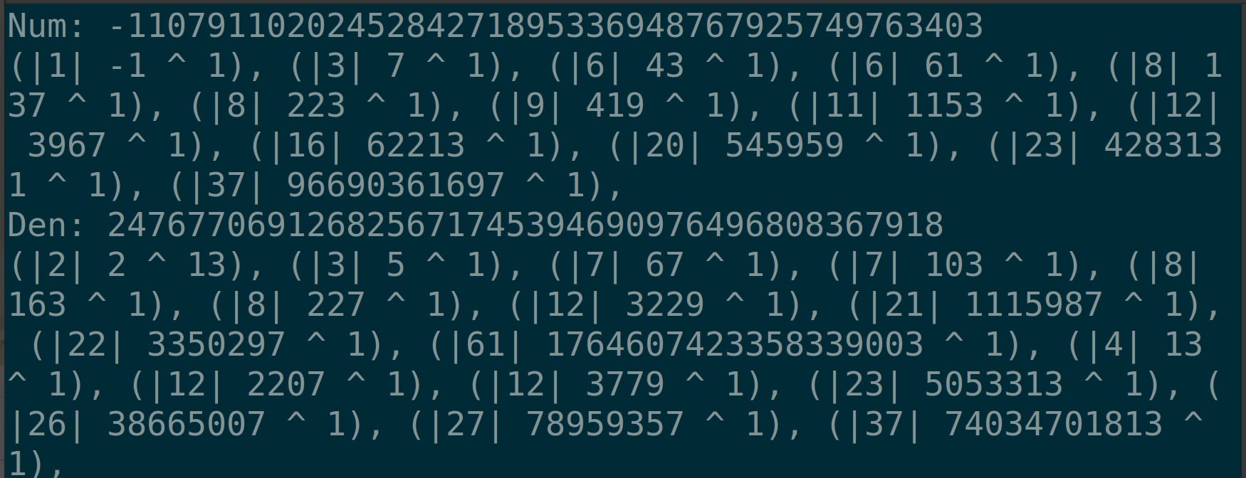
and observe the factorization (after running for a second):
Two things can happen now: either run the sieve longer or split the primes over a number field like in the Gaussian Integers paper.