Chebyshev Polynomials and Their Derivatives in C

Quick Summary

We use the C language to observe the incredible features of chebyshev polynomials: orthogonality. easy-to-find approximations, and even easier-to-find derivatives.

We provide Python starter code and complete C code (15 June update) at these links.

Numerical analysis is the design of computer algorithms to solve math and physics problems (Shi, 2024)1.

Chebyshev polynomials are like ferraris among numerical analysts because they are fast, precise and the math is beautiful.

This article serves as a friendly introduction to chebyshev polynomials for programmers.

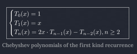
In approximation theory, Chebyshev Polynomials are sequences of polynomials defined on the interval [-1, 1] that satisfy the recurrence (Sidharth et al., 2024):

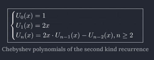
Chebyshev polynomials of the second kind satisfy the recurrence:

Chebyshev polynomials possess these properties:

1. Orthogonality:

   • The chebyshev polynomials of the first kind form a set of orthogonal polynomials over the real interval [-1, 1] (Mason & Handscomb, 2023)2.

   • Being orthogonal ensures the polynomial coefficients are uncorrelated for convergence and numerical stability (Sidharth et al., 2024).

2. Recursive definition:

   • This we observed in the definition of chebyshev polynomials.

3. Inversion symmetry (Deus Ex Machina, 2021)3:

   • This means that T_n(x) = T_n(-x)

4. Rapid Convergence and Uniform Approximation (Sidharth et al., 2024):

   • The approximation error of chebyshev polynomials decreases faster than other polynomial bases as degree increases.

   • Compared to same-degree polynomials, chebyshev polynomials minimize better the maximum approximation error.

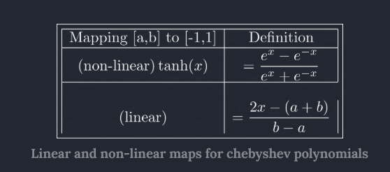
5. Easy to map:

   • Chebyshev polynomials on the general interval [a,b] can be mapped to the real interval [-1,1] either:

     • non-linearly using the hyperbolic tangent (Sidharth et al., 2024)

     • by a simple linear map (Bray, 2016)4:

       

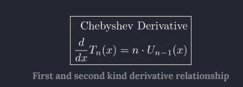
6. Easily differentiable:

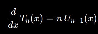
   • The derivative of the n-th chebyshev polynomial of the first kind is equal to n times the (n-1)-th Chebyshev polynomial of the second kind.

     

Chebyshev polynomial expansions help programmers find solutions to differential equations.

Say you want to find the solution u to a differential equation. You’d find the chebyshev expansion coefficients u_k alongside a set of weights ϕ_k . We saw this in the Chebyshev KAN paper implementation.

Chebyshev polynomials are part of a broad class of algorithms for solving differential equations called spectral methods.

Formulating a spectral method involves finding trial functions (also called expansion or approximating functions) and their test functions (also known as weight functions) (Canuto, 2006)5.

In the case of chebyshev polynomials, one obtains trial and test functions using cosine transforms or backpropagation with KANs:

This is a coding section. We offer Python starter code here but the rest of the article is in C.

Finding Chebyshev expansion coefficients is called interpolation with Chebyshev polynomials. We interpolate in the canonical basis.

The canonical basis expresses the Chebyshev polynomial of the first kind as a sum of increasing powers:

So interpolation refers to us finding the coefficients in the equation above.

We can visualize the canonical basis of chebyshev polynomials in Python:

import numpy as np
from numpy.polynomial.polynomial import polyval
import matplotlib.pyplot as plt

def ChebyshevRecurrence(N):
    coeffs = np.zeros((N + 1, N + 1))
    coeffs[0, 0] = 1
    coeffs[1, 1] = 1
    for k in range(2, N + 1):
        coeffs[k] = 2 * np.insert(coeffs[k - 1, :-1], 0, 0) - coeffs[k - 2]
    return coeffs

def ColorList(n):
    cmap = plt.get_cmap(’tab10’)
    return [cmap(i % 10) for i in range(n)]

def PlotChebyshevPolynomials(N, x_range=(-1, 1), num_points=400):
    coeffs = ChebyshevRecurrence(N)
    x = np.linspace(x_range[0], x_range[1], num_points)
    colors = ColorList(N + 1)
    fig, ax = plt.subplots(figsize=(8, 5))
    for k in range(N + 1):
        y = polyval(x, coeffs[k])
        ax.plot(x, y, lw=1.5, color=colors[k], label=fr’$T_{{{k}}}(x)$’)
    ax.set_title(fr”Chebyshev Polynomials $T_0(x)$ to $T_{N}(x)$”, fontsize=14)
    ax.set_xlabel(”x”)
    ax.set_ylabel(”Tₙ(x)”)
    ax.grid(True)
    ax.legend(loc=’upper right’)
    plt.tight_layout()
    plt.show()


numberOfPolynomials = 3
PlotChebyshevPolynomials(numberOfPolynomials)

Running this code yields the image below. Observe how the lines rarely intersect.

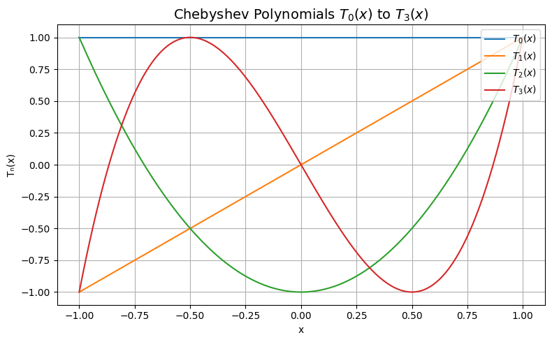
The image above demonstrates the orthogonal nature of chebyshev polynomials and why they’re great basis functions.

As mentioned earlier, one can find expansion coefficients by backpropagation.

However, a faster technique exists and it’s called Lagrange interpolation at Chebyshev-Gauss-Lobatto (CGL) points.

In a nutshell, one identifies special points then attempts to fit a chebyshev polynomial through these points.

A more formal definition is provided below (Combette GitHub, 2023)6:

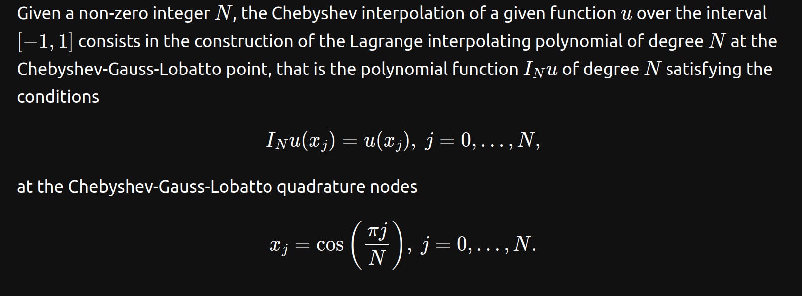
The Chebyshev-Gauss-Lobatto quadrature nodes introduced above are the extrema of the chebyshev polynomial on the interval [-1,1].

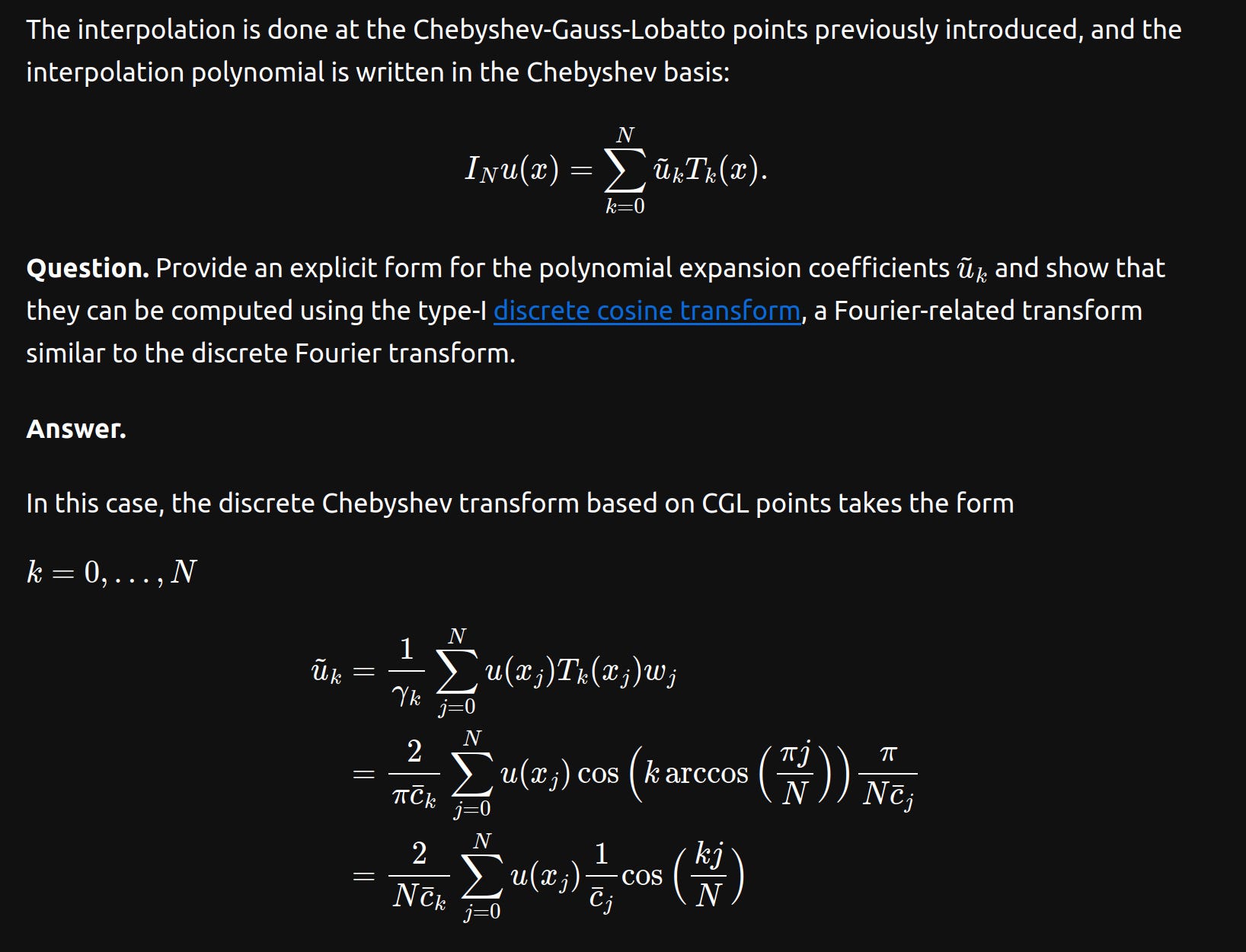
One first identifies the CGL points then proceeds to fit a chebyshev polynomials using the Type-I Discrete Cosine Transform.

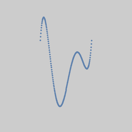
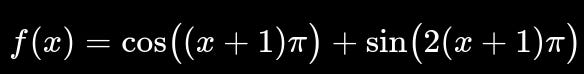
Say we desire to approximate the function below:

First, we define a struct to hold our Chebyshev data:

typedef struct chebyshev_sampler_struct *Chebyshev;
struct chebyshev_sampler_struct
{
	int degree;
	int stride;
	float *chebyshevGaussLobattoNodes;
	float *samples;
	float *coefficientsDCT1;
};

where:

• Degree: the degree of our chebyshev polynomial.

• Stride : this is degree + 1.

• chebyshevGaussLobattoNodes: These are the locations where we sample the original equation.

• samples: These are the values of the original equation at the chebyshevGaussLobattoNodes.

• coefficientsDCT1: Here we store the results of passing samples through the DCT-Type 1.

Once we load our samples, we pass them through a DCT-Type 1:

//https://docs.scipy.org/doc/scipy/reference/generated/scipy.fft.dct.html
void FindDCTTypeIForward(int length, float *input, float *output)
{
	for(int i = 0; i < length; i++)
	{
		float temp0 = input[length-1];
		if(i % 2 == 1){temp0 *= -1;}
		float temp1 = 0;
		for(int j = 1; j < length-1; j++)
		{
			float temp2 = cos((M_PI * i * j) / (length - 1));
			temp2 *= input[j];
			temp1 += temp2;
		}
		output[i] = input[0] + temp0 + 2 * temp1;
		
		//normalize
		output[i] /= 2 * (length - 1);
	}
}

Note that in this DCT implementation, we need to double the inner coefficients after applying the transform:

//Call DCT Type 1
FindDCTTypeIForward(chebyshev->stride,chebyshev->samples, chebyshev->coefficientsDCT1);

//Double inner coefficients after applying the transform
for(int i = 1; i < chebyshev->stride-1; i++){chebyshev->coefficientsDCT1[i] *= 2;}
	

After applying the DCT-I, we sample the chebyshev polynomial. We provide an input x and this function tells us the corresponding y:

float ChebyshevApproximationFast(Chebyshev cheby, float x)
{
	assert(x >= -1.0f);
	assert(x <= 1.0f);
	float theta = acosf(x);
	float result = 0.0f;
	for(int k = 0; k < cheby->stride; ++k)
	{
		float Tk = cosf(k * theta);
		result += cheby->coefficientsDCT1[k] * Tk;
	}
	return result;
}

We put everything together and get this:

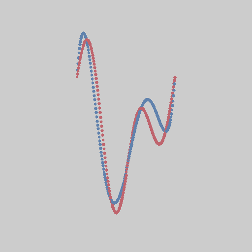
The blue dots are what we wanted to approximate. The red dots are our predicted positions for a degree 5 polynomial.

If we increase the degree of our chebyshev polynomial to 15, then we get a perfect match!

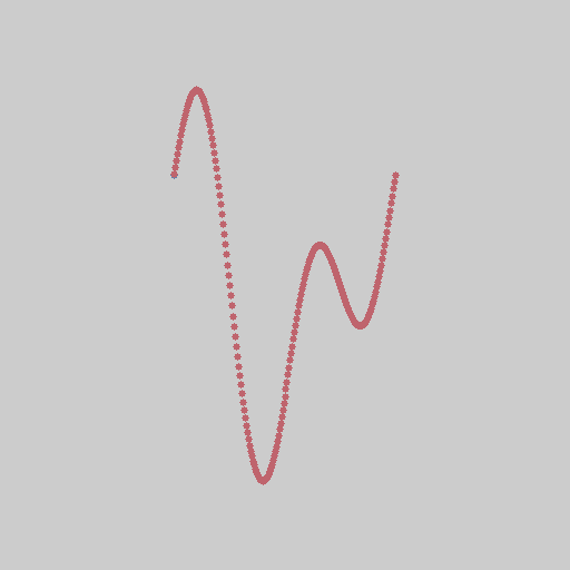
The example is the polynomial cos((x+1) * PI) + sin(2 * (x+1) * PI) and a degree 15 chebyshev approximated it perfectly!

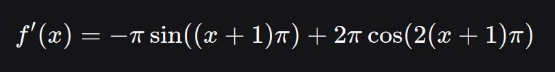
Earlier, we revealed that the sampled equation was:

Its derivative is:

Here’s a neat fact about chebyshev polynomials: we can differentiate the approximate coefficients (pretty fast) to obtain the derivative.

We start with the identity: the derivative of the n-th chebyshev polynomial of the first kind is equal to n times the (n-1)-th Chebyshev polynomial of the second kind.

We further know the identity relating the chebyshev polynomials of the first and second kind:

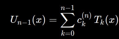
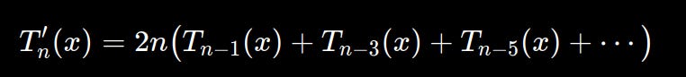
We substitute this to observe the wildest thing: we can recursively sum our DCT coefficients to obtain the approximate derivative.

The C code for this resembles:

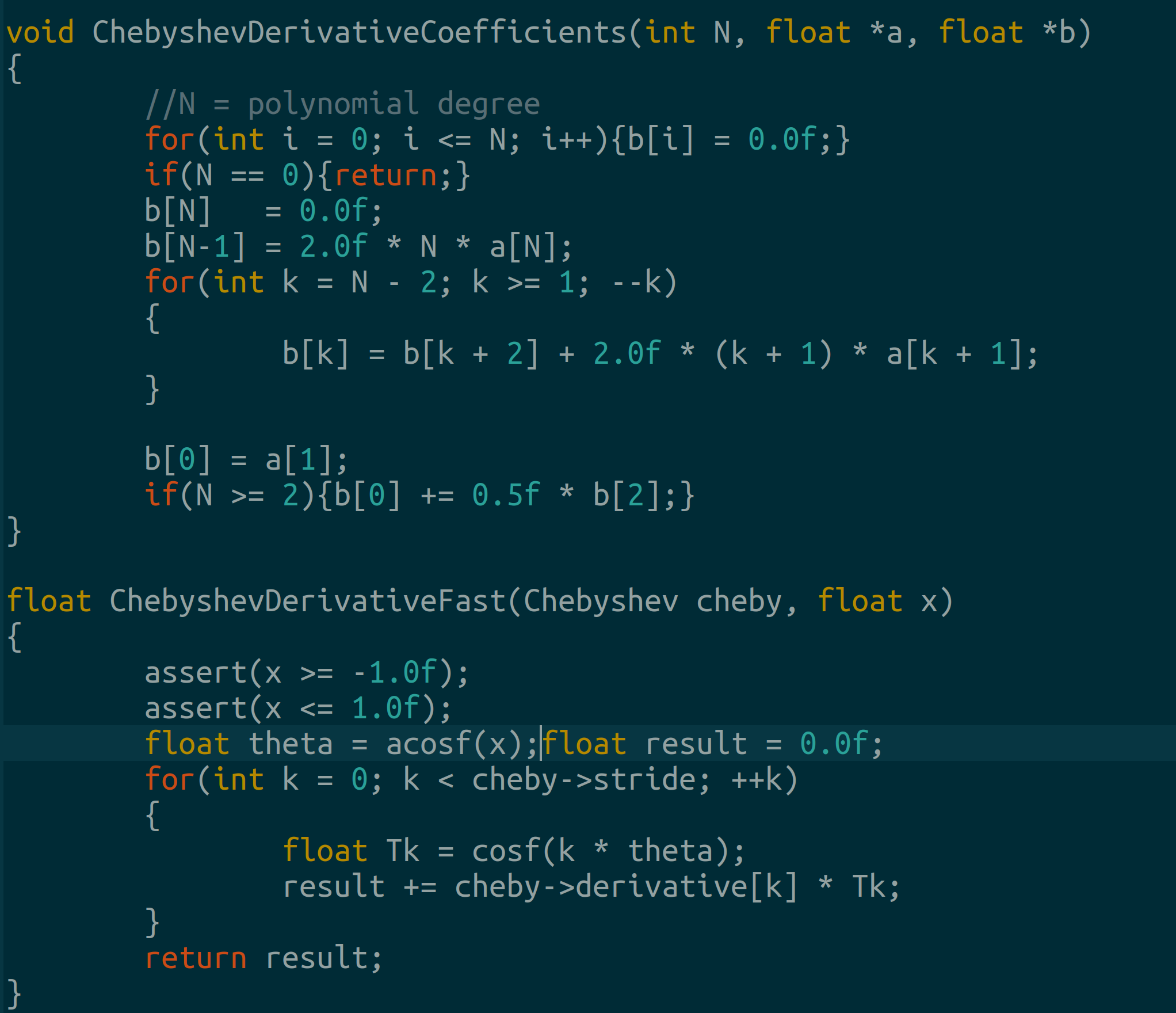
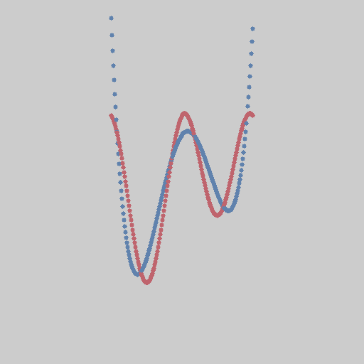
The degree 5 chebyshev polynomial’s recursive derivative almost matches the target polynomial derivative:

At degree 10, our derivative matches almost perfectly!

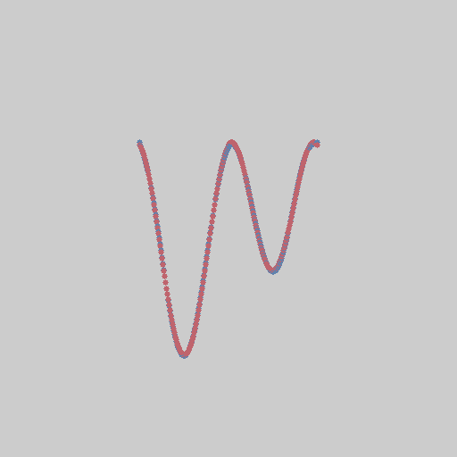
Imagine that! We found the derivative without needing an upstream gradient.

Chebyshev polynomial interpolation is amazing. However, there is no free lunch due to:

1. Gibbs phenomenon: polynomials overshoot when a function has jumps or is discontinuous. (Herman, 2025)7

2. Runge phenomenon: extreme oscillations at the endpoints when the function to be approximated has equidistant nodes.(Cook, 2017)8

   • Some clever guys invented Chebyshev-Gauss-Lobatto (CGL) nodes to handle this (Combette, 2023)9

     

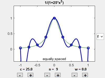
These problems tend to occur but they’re super manageable.

Chebyshev polynomials also turn up in interesting places:

• In AI, Chebyshev polynomials are a basis for Kolmogorov Arnold neural networks as described in (Sidharth et al., 2024).

• In Number theory, every valid solution to Pell’s equation defined over a finite field can be represented by chebyshev polynomials of the first and second kinds(Barbeau, 2003)

We can extend this to do other things. For instance, AI researcher build Kolmogorov-Arnold Networks using Chebyshev Polynomials.

Here are some free gpu credits if you made it this far lol.