In a recent article, I brought up an important gotcha about electricity:
“In electronic circuits, the flow of electrons is confined to conductors, but the transfer of energy doesn’t involve these particles bouncing off each other; instead, the process is mediated through electromagnetic fields. These fields originate from charge carriers, but extend freely into the surrounding space.”
This property stumps many novices, especially if they cling on to the didactical toll known as the hydraulic analogy. Without considering interactions at a distance, it’s hard to grasp the behavior of transistors, capacitors, inductors, and other electronic components.
But how do these fields behave? The electric field is the easy one: most simply, it’s the static force of attraction and repulsion between charge-bearing particles. It’s what binds electrons to the nucleus of an atom, and what causes packing peanuts to stick to cats.

Magnetic fields are more mystifying. Most textbooks assert that they’re a manifestation of the same underlying phenomenon, but then proceed to treat them as as wholly separate animal governed by its own, seemingly ad-hoc rules. The authors reach into a hat and pull out a “B field” or an “H field” that acts on moving particles… but only when the textbook says it should.
To develop better intuition, we ought to start with the speed of light. The significance of the concept is sometimes misunderstood, but in the most basic sense, it appears to be a fundamental constraint on causality: you can’t exert influence at a distance any faster than it would take for a photon — a massless elementary sorta-particle — to travel from here to there.
This creates an interesting problem for Newtonian physics. Let’s imagine that a guy named Finn is sitting near the front of railroad car that’s 60 feet long and driving past at 90% the speed of light:

Conventionally, the the frame of reference of an observer standing in a nearby meadow is as good as Finn’s; in fact, Finn might argue that he’s stationary and the lamp is getting away. There should be nothing unusual about physics onboard his car, and from Finn’s perspective, it stands to reason that light from the lamp should be reaching him at roughly t + 60 nanoseconds: that’s how long it takes for photons traveling at the speed of light to clear the length of the car.
But from your frame of reference, this ain’t right! By the time the photons travel 60 feet, the front of the car has moved by over 50 feet. Either Finn’s photons are a lot faster than yours, or more time needs to pass before they reach him.
An early attempt to address this issue was the concept of luminiferous aether: a cosmic medium through which photons supposedly propagate at a constant speed. This theory implied the existence of a special, “aether-anchored” frame of reference. If that happened to be your frame, then Finn, tearing through the aether at breakneck speeds, would see the physics on his railroad car getting out of whack.
Alas, no proof for the existence of luminiferous aether could ever be produced; instead, the answer turned out to be special relativity. The theory posits that, yes, all inertial frames of reference are equivalent. Instead, the trick is that when the frames are in relative motion, they experience space and time in different ways. In particular, in our frame of reference, instantaneous measurements of Finn’s car would indicate it’s shorter than expected, and the time onboard would be seemingly passing more slowly than in the meadow we’re at.
To offer a basic explanation of magnetism, we really only need to lean on relativistic length contraction: the apparent reduction of the size and distance between moving objects along the direction of their travel. The effect is negligible in most contexts unless the objects are moving at very high (“relativistic”) speeds, but electric fields are a notable exception. The average drift speed of electrons in a wire usually doesn’t exceed several centimeters per minute, but there’s a great number of them, and the fields are powerful: two coulomb charges placed one meter apart repel with the force equivalent to 900,000 metric tons!
To get going, let’s consider a section of copper wire at rest. In the metal, there’s a certain number of mobile electrons in the conduction band, skating across a lattice with a matching density of immobile, positively-charged copper ions. Internal electric fields require the electrons to stay in the conductor, but they’re not kept on a particularly tight leash:
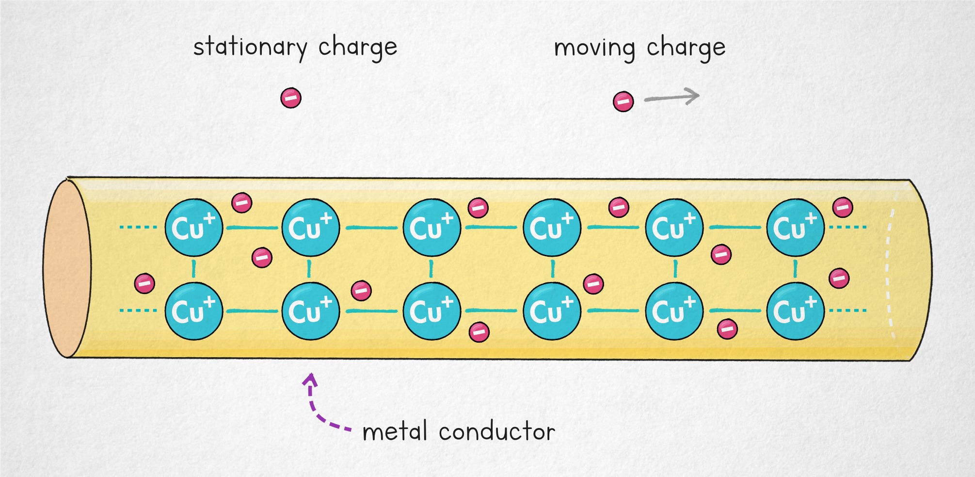
In this setup, because the positive and negative charges in the conductor are in balance, there is no net electric field acting on the two stray charges pictured nearby, regardless of whether they’re moving or not.
For the next step, it’s helpful to imagine a toy circuit: a one-meter loop of wire with one hundred mobile electrons inside. It’s a simple necessity that in the stationary (“lab”) frame of reference, the average distance between these electrons stays constant — 1 cm — no matter if the’re staying put or circulating around the loop. The only way to change their spacing would be to add electrons or take away some; otherwise, it’s always 100 elementary particles spread throughout a meter of wire.
But electrons in motion must undergo some length contraction! That is to say, once they start moving in relation to the observer, their apparent spacing in the direction of travel ought to be tighter than the “true” distance in the electrons’ frame of reference. The only way to square this is to realize that the electrons in motion must be spreading out in their frame of reference; there is no requirement that the length or shape of the loop of wire remains the same from the point of view of the moving charge.
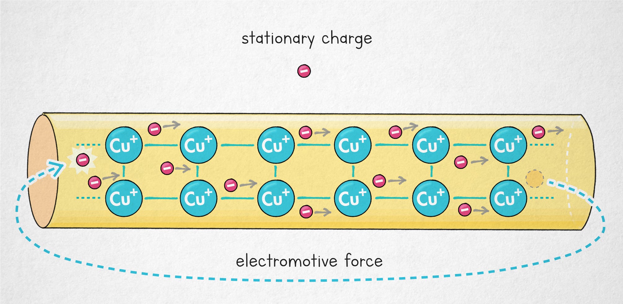
With this in mind, let’s revisit the earlier conductor model, this time with some current flowing through. As we established earlier, in the lab frame of reference, the conductor is not getting any shorter or any longer, so the (notionally length-contracted) density of electrons and copper ions stays in balance. Because of this, there is no net electric field acting on a nearby stationary charge:
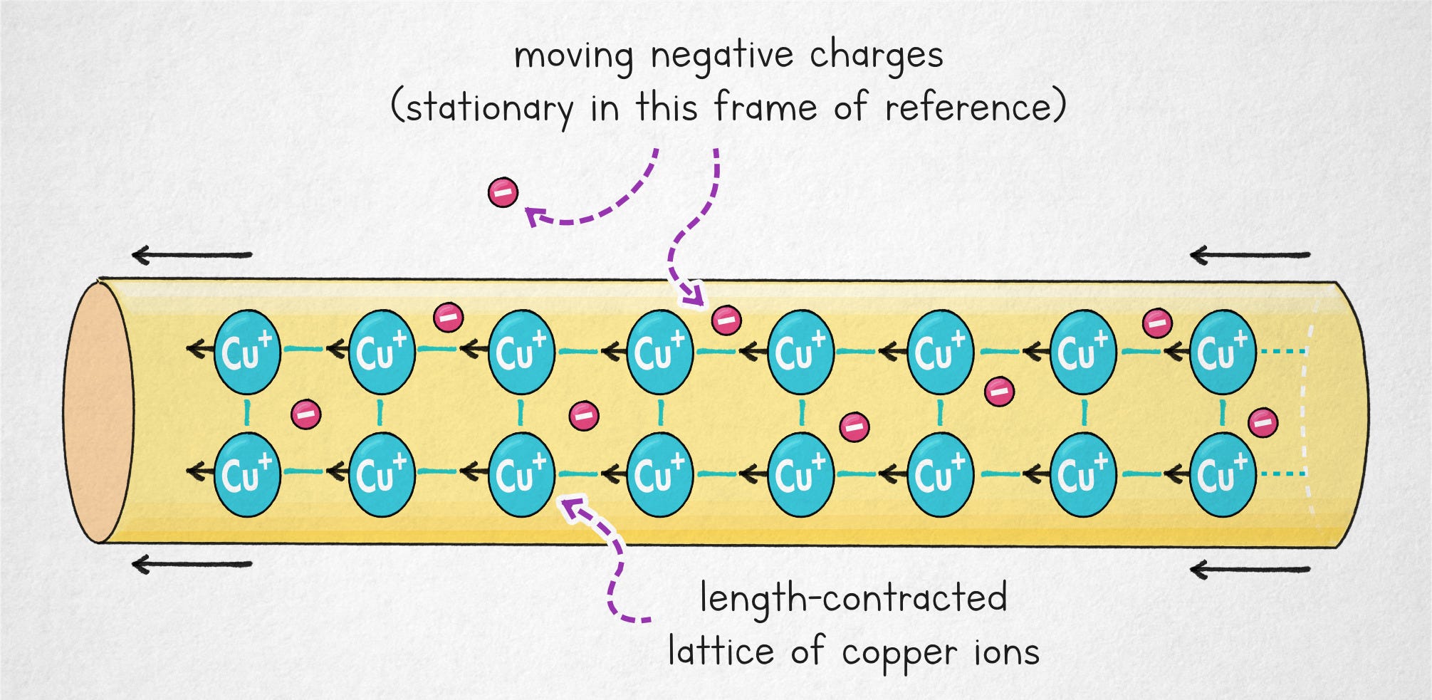
But what about a random charge outside the conductor that’s traveling in the same direction as the electrons inside the wire? Well, from its perspective, the conductor consists of a bunch of non-moving electrons spaced pretty far apart, and then a markedly higher density of positive ions moving the other way round!
In other words, the charge, in its frame of reference, would experience a net electric field that’s pulling it toward the conductor — but again, only if it was moving along it in the first place:
And this is, in essence, the origin of magnetic fields. Or, more properly: it’s a way to show that they arise as a natural consequence of electrostatic interactions. We’re not giving either of the phenomena a claim to primacy, because one could start with magnetic interactions and from that, derive electrostatic fields.
It’s not always useful to analyze the effect this way. In particular, the model gets less intuitive for accelerating charge carriers and the interactions with permanent magnets. In the first case, common-sense solutions exist, just take more effort to derive. In the second case, the conceptual problem is that electron spins don’t have a clear-cut analog in the macroscopic world, so folksy explanations get stretched really thin.
Still: it’s good to have a slightly more intuitive explanation of where this mysterious force comes from.
👉 For further articles about electronics, click here.
I write well-researched, original articles about geek culture, electronic circuit design, algorithms, and more. If you like the content, please subscribe.