A key challenge when equipping agents with a large number of tools is that the agent often cannot reliably determine which tool to choose, especially when the tool set is large. Protocol‑based layers such as Model Context Protocol (MCP) attempt to standardize tool access, but even for them, there is a natural limit. It’s less than 50.
In enterprise settings where a vast number of APIs may be available, such constraints become showstoppers. I am currently working with a bank that has thousands of APIs across several parts of the company. How do you handle agentic tool discovery then? This problem is amplified when you lack strict discipline or governance to define clear boundaries around agent permissions and responsibilities.
For most Agent implementations the standard approach of defining tools is a list. And this is what most agent frameworks provide when configuring an agent. That approach, while simple, is inherently brittle; it does not scale well and is prone to misconfiguration, redundancy, and errors.
In this article, I will talk about another way, maybe a more effective way, to let agents discover themselves the right tool to use. Especially interesting for you might be that in this case, tool discovery is handled through a knowledge graph.
Let’s dive right in.
As I already have shown here, here, here and here while talking about graph reasoning, knowledge graphs represent structured information in the form of a graph. They consist of Nodes, which usually represent entities like people, places, and things, and also edges that represent relationships between these entities.
But there is more.
Among the components is also the schema which defines the types of entities, their attributes, and relationships between the entities. In that sense, the schema defines the general layout of the knowledge graph while the instance data then actually form the graph following the definitions of the schema.
In short, the schema defines what can exist; the instance data defines what does exist.
Within the context of this chapter, I want to introduce two GDM models. One is the labelled property graph (LPG), the other is the Resource Description Framework (RDF). Both are popular data models often used in graph databases like Neo4J, but they cater to different use cases and have unique strengths.
LPG amends the previously introduced Node/Edge description with the concept of
(a) Properties. Key-value pairs are stored on nodes or relationships. The goal here is to provide additional metadata describing the node/edge combination.
(b) Labels to classify nodes and edges into categories or types. I like to think of them as clusters.
Among the benefits of LPG is that schemas can flexibly be adapted and can perform graph traversals incredibly fast.
RDP, on the other hand, is a W3 semantic web standard that applies a standardized data model to represent information as a collection of triples (subject – predicate – object). The grammatical nature of this structure is obvious. RDF is schema-first. That means, all relationships and entity types in the graph follow strict, machine-interpretable definitions defined in vocabularies/ontologies such as RDFS or OWL. While RDF data forms a directed labelled graph, metadata in form of properties attaches itself to entities indirectly via additional triples. RDF is not necessarily the fastest in graph traversal, as it excels in knowledge representation, interoperability, and logic-based reasoning. I used it in the past mostly for large, interconnected knowledge graphs where consistency, inference, and linking across datasets matter more than the performance of operational graph queries. Finally, RDF does not enforce a schema.
What SQL is to relational data model of databases, is SPARQL to RDF. A standard query language for RDF documents will have well-defined semantics.
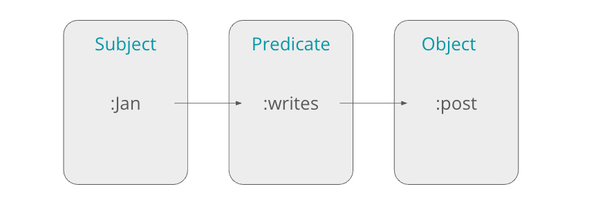
Within the context of the RDF, we use unique resource identifiers (URI) to uniquely identify resources within the graph. We can add attributes to the resources. I.e., Jan is a person and author. Post could be Substack, Text.
RDF graphs are usually presented in a machine-readable format.
Now, how do we construct knowledge graphs?
Let’s start with the data.
Data to construct a knowledge graph can come in many shapes or forms.
Structures sources: R2RML
Semi-structured: Flexible schemas like XML
Unstructured: Natural language texts, images.
For this, we first need to create descriptive data about the APIs, then we analyze the raw data that we have received and validate the data quality. Then we model the clean data into standardized RDF triples. The final step is then generating the knowledge graph.
When directing cognitive agents to discover APIs as tools to use, giving the right context increases reliability substantially. Especially if you consider that in many organizations, there are thousands of different APIs that might be relevant. What we want to do is to create a knowledge graph of the APIs and enrich it with domain-specific process information. This should help guide the agent. It is time and cost-prohibitive to task an agent to discover the right API for every call. And, narrowing down the search space through directed acyclic knowledge graphs can make this planning exercise much more efficient.
Secondly, when you consider retrieval systems like RAG, then you will notice that they often miss the deeper structure and content. Also, LLMs are still quite poor at rule-following. KGs can ingest process context and also up-to-date metadata into the agent’s context, reducing hallucinations.
Also, for building trust, auditable knowledge graph paths are easier to trace.
Let’s make this a bit more concrete.
When agents operate inside an enterprise, the practical bottleneck is rarely model quality. It is almost always tool selection. Once the number of available tools passes a few dozen, the agent’s decision space becomes noisy. As mentioned, MCP has one major disadvantage. It pollutes the context window with a lot of tokens that might hardly ever be used. Not only for that reason is the number of MCP tools finite.
Since static tool lists don’t scale well, and manual curation doesn’t keep pace with organizational entropy, I believe a different pattern is needed.
A knowledge graph provides that pattern.
Consider a typical financial data environment.
It might include APIs like these:
By right, each API serves its own subgraph of the information topology: news streams, market ticks, fundamentals, sentiment, and institutional data.
I want to make sure that I call the right API at the right time for the right intent.
Something like this:
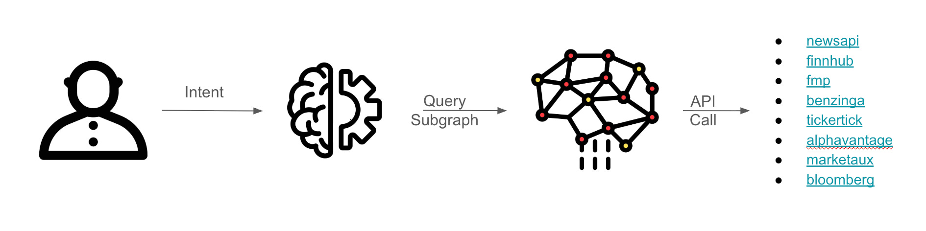
In that sense, the difference between automation and orchestration is that now automation evolves from “How do I call them?” to the orchestrative “Which one fits the current intent?”. Through that, the problem becomes a classification problem, not a parsing problem. And not coincidentally, classification is what graphs are really good at.
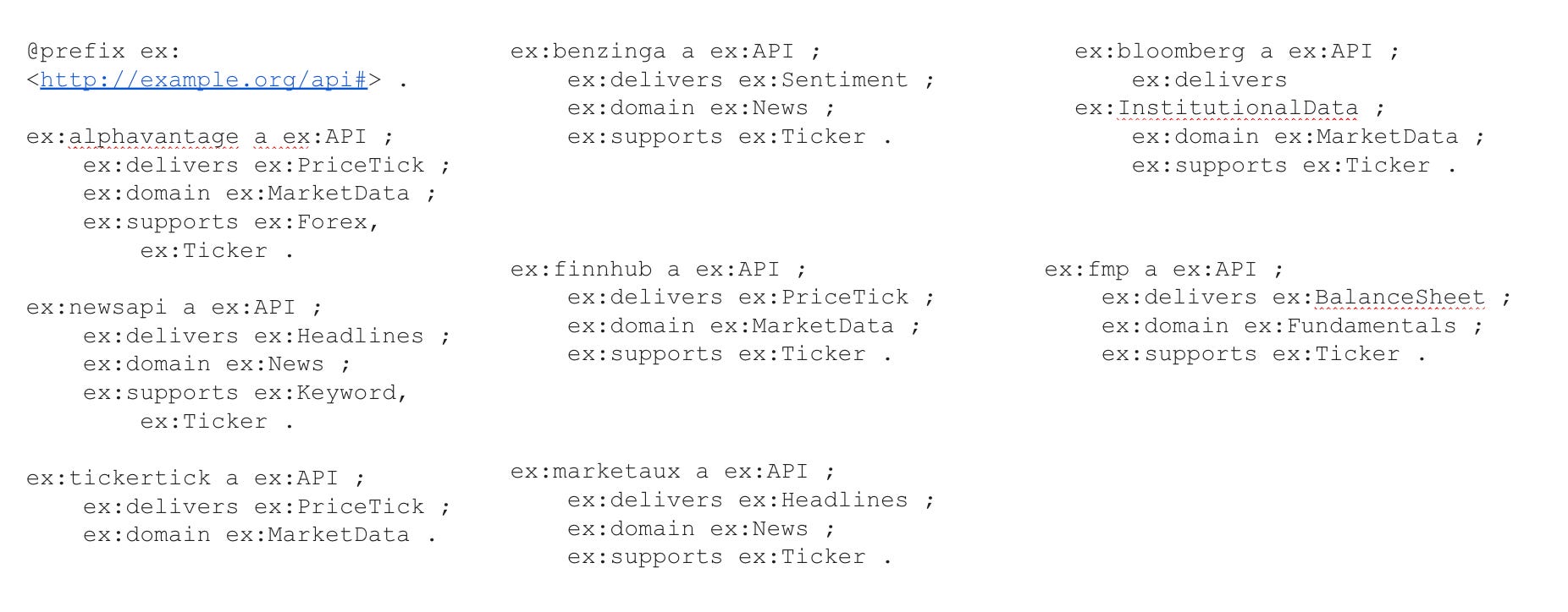
Now using RDF, we can deconstruct each API definition into semantic components.
To do this, we must describe each API as a collection of triples consisting of:
its functional domain (e.g., News, MarketData, Fundamentals)
the type of data it emits
what query structures it supports
any constraints around usage
A fragment for newsapi might look like this:
:newsapi        rdf:type       :API .
:newsapi        :domain        :News .
:newsapi        :delivers      :Headlines .
:newsapi        :supports      :Ticker .
This might appear trivial for now, but scale it to hundreds of tools and the graph starts acting as a map of capabilities.
The next step is then to start constructing the representation of the knowledge graph. Here we will be using rdflib’s onboard toolkit. The concept is quite simple.
The “add_api” function constructs the graph by adding nodes and edges to it.
from rdflib import Graph, Namespace, Literal, RDF

EX = Namespace(”http://example.org/api#”)

g = Graph()
g.bind(”ex”, EX)

def add_api(identifier, domain, delivers, supports=None):
    api = EX[identifier]
    g.add((api, RDF.type, EX.API))
    g.add((api, EX.domain, EX[domain]))
    g.add((api, EX.delivers, EX[delivers]))
    if supports:
        for s in supports:
            g.add((api, EX.supports, EX[s]))
    return api

# APIs (no version tags)
add_api(”newsapi”,“News”,“Headlines”,[”Ticker”, “Keyword”])
add_api(”finnhub”,“MarketData”,“PriceTick”,[”Ticker”])
add_api(”fmp”,“Fundamentals”, “BalanceSheet”,[”Ticker”])
add_api(”benzinga”,“News”,“Sentiment”,[”Ticker”])
add_api(”tickertick”,“MarketData”,“PriceTick”)
add_api(”alphavantage”,“MarketData”,“PriceTick”,[”Ticker”, “Forex”])
add_api(”marketaux”,“News”,“Headlines”,[”Ticker”])
add_api(”bloomberg”,“MarketData”,“InstitutionalData”, [”Ticker”])

print(g.serialize(format=”turtle”))
This produces a minimal but expressive graph, enough structure to guide an agent, without burying it in ontological ceremony.
So, what is the value added to represent the graph using RDF?
Well, for once we can query the graph and extract subgraphs. So, instead of handing and maintaining 50+ tools in context and let the agent decide which one to select, we can now apply a deterministic semantic filter first.
We use SparQL for this. Below are a two examples how this should work. Btw, the question mark in the below query indicates a variable. The rest is like standard SQL.
Task: retrieve all APIs that produce price ticks.
from rdflib.plugins.sparql import prepareQuery

q = prepareQuery(”“”
PREFIX ex: <http://example.org/api#>
SELECT ?api WHERE {
    ?api ex:delivers ex:PriceTick .
}
“”“)

for row in g.query(q):
    print(row.api)
Typical response then should be:
.../finnhub
.../tickertick
.../alphavantage
.../bloomberg
Task: Which APIs provide news and accept ticker-based queries?
q = prepareQuery(”“”
PREFIX ex: <http://example.org/api#>
SELECT ?api WHERE {
    ?api ex:domain ex:News ;
         ex:supports ex:Ticker .
}
“”“)

for row in g.query(q):
    print(row.api)
Expected output:
.../newsapi
.../benzinga
.../marketaux
The agent now has a clear, bounded candidate set, reducing the hallucination of nonexistent tools or misinterpreting names.
I observed that this approach works for three main reasons:
Stable semantics
Tools evolve, but their functional categories rarely do.
RDF captures those categories cleanly.Auditable reasoning
Semantic filter produces paths in text form.
You can inspect exactly why a tool was chosen. Its an important reliability criteria.Composable environment design
Adding new APIs means adding triples into the graph. Not modifying agent code.
Therefore, this shifts tool use from ad-hoc selection to structured inference.
The agent navigates the space of capabilities the same way a compiler navigates a type system through a graph of constraints and affordances.
To leverage the full value of a knowledge graph (KG) of APIs not only for discovery, but for full planning, execution and dynamic adaptation, we can embed a planning loop over the graph. This transforms tool usage from ad‑hoc calls to a structured, dependency-aware execution plan.
Let us therefore define a planning graph structure first. Similar to what we have seen above in the general graph structure, we need 3 things.
State graph: represents the agent’s current context/objectives/constraints.
Action graph: represents possible tool-invocation actions (API calls), where each action has preconditions (what we know so far) and effects (what new data or state will result).
Dependency edges: show which actions require the results of which prior actions. In effect, the graph captures a partial‑order plan rather than a fixed sequence.
This pattern is similar to classical planning graphs used in AI planning (alternating state and action levels, with mutex constraints) when exploring STRIPS‑like planning problems.
With this structure, the agent now can:
Expand the graph to enumerate candidate actions whose preconditions are satisfied;
Select among actions based on heuristics or metadata (cost, latency, licensing, reliability, domain constraints);
Execute one or more actions (possibly in parallel if independent);
Observe results and update the state;
Repeat until goal is reached or no further actions viable.
This loop is naturally a graph-based planning loop, not a linear script, but a dynamic, data-driven, dependency-aware plan.
Building and running a knowledge‑graph (KG) of APIs is appealing due to its easy to understand visual representation and low footprint. If you consider real enterprise production needs, you face a number of non‑trivial operational questions.
In short, things change.
API changes, new endpoints, deprecations. APIs rarely stay static. Endpoints may change, parameters may evolve, response formats may shift, or entire APIs may be deprecated. To reflect that in your KG, you need a maintenance pipeline. For example: periodically fetch OpenAPI / Swagger specs (if available), parse them, then diff against your KG to insert new triples (new endpoints), update existing metadata, flag deprecated ones.
Schema drift and backward compatibility. Suppose you previously declared that Bloomberg delivers BalanceSheet information. What if future versions add new data types (e.g. cashflow, ESG) or change naming? Your KG schema may need to evolve. This means you need versioned metadata and not just “this API” but “this API@timestamp/version”.
Automated vs manual updates. For public APIs with open specs (OpenAPI, GraphQL introspection, etc.), you might script automated ingestion. For proprietary or internal APIs, manual metadata maintenance may be unavoidable. Having a governance process around API onboarding and deprecation becomes necessary.
Thus, the KG isn’t “write once, forget forever.” It requires ongoing maintenance. Ideally with automated spec‑scraping + human validation + versioning.
So, how to approach this?
Versioning & deprecation.
When an API releases a new version, your KG should reflect that. One pattern: treat each distinct version as a separate node/resource in the graph (e.g. fmp_v3, fmp_v4), with relationships like :isSuccessorOf, :isDeprecated, :supersedes. Agents can then choose only non‑deprecated nodes, or optionally allow legacy ones if flagged. The most straightforward way should be to add this to the SparQL semantic filter. This would also help with inconsistencies in versioning between the KGs.
Rate limits, quotas, latency, and reliability metadata.
These are essential for real-world usage but often overlooked in toy examples. You should augment your KG with attributes like :rateLimitPerMinute, :costPerRequest, :typicalLatencyMs, :licenseRequired, etc.
That way, planning can take not just functional capabilities but also non‑functional constraints into account (e.g. “don’t pick API if rate‑limit close to exceeded,” or “choose lower-latency API for real-time tasks”).
Fallback & redundancy.
If your agent picks API A but it fails (timeout, error, rate limit), the KG + planning logic should allow fallback: pick API B offering the same data type. That requires metadata about overlapping capabilities. You should also consider that the data mappings from the source then are likely different.
In many popular examples, authentication, credentials, and security are often forgotten. Therefore, it is important to at least have an understanding of the problem statements here.
Credential management. Many financial APIs require API keys, OAuth tokens, or enterprise licenses. Your KG should not store raw credentials (security risk), but should store metadata about required credentials (e.g. :requiresApiKey = true, :licenseType = “enterprise”). The actual credentials should live in a secure vault or environment variable store.
Access control and governance. In regulated settings, you may want to enforce policy: e.g. only certain agents (or users) may call paid APIs, or only under certain conditions. Embedding such policy metadata in the KG, or in an overlay policy graph, helps: e.g. :apiKeyOwner, :allowedEnvironments, :dataRetentionPolicy.
Agents can check these before invoking.
Audit trails & logging. When the agent calls an API, you should log which API node (and version) was used, timestamp, response status, user/agent identity, so that for compliance or debugging, you can reconstruct. The KG helps because it adds semantic identity (not just a URL string but a node you can refer back to).
As you know, I am still quite fond of Huggingface’s Smolagents library.
Here is a sketch of how one might integrate the above outlined planning loop, combining your RDF API‑KG and the KG-based plan as a “planner + executor” module inside a CodeAgent.
from smolagents import CodeAgent, tool, InferenceClientModel
from rdflib import Graph, Namespace, Literal, RDF
from rdflib.plugins.sparql import prepareQuery

# --- Build (or load) your API knowledge graph ---
EX = Namespace(”http://example.org/api#”)
kg = Graph()
kg.bind(”ex”, EX)
# ... (add APIs as shown in earlier examples) ...

# Example tool wrapper for making an API call — the agent can call this.
@tool
def call_api(api_name: str, payload: dict) -> dict:
    # A generic dispatcher: depending on api_name, encode and send request, return JSON/dict
    # For simplicity, place holder logic; in real code route to actual client (requests / SDK)
    print(f”Calling {api_name} with {payload}”)
    return {”dummy_response”: True}

def plan_and_execute(goal: str):
    “”“
    Pseudocode: 1) query KG for candidate APIs that satisfy the goal
                2) pick, call, observe; repeat if needed.
    “”“
    # Example SPARQL — find APIs delivering price ticks if goal involves ‘price’
    q = prepareQuery(”“”
    PREFIX ex: <http://example.org/api#>
    SELECT ?api WHERE {
      ?api ex:delivers ex:PriceTick .
    }
    “”“)
    apis = [str(row.api) for row in kg.query(q)]
    # pick first for demo
    chosen = apis[0] if apis else None
    if chosen:
        resp = call_api(chosen, {”symbol”: “AAPL”})
        return resp
    else:
        return {”error”: “no suitable API found”}

# Instantiate a CodeAgent that can use this planner
model = InferenceClientModel()  # or any compatible LLM backend
agent = CodeAgent(
    tools=[call_api],
    model=model,
    stream_outputs=True
)

prompt = “”“
Task: retrieve the latest price tick for symbol “AAPL”.
You have access to a knowledge‑graph of APIs. First plan which API to call, then call it via `call_api`.
“”“
agent.run(prompt, additional_context={”kg”: kg, “planner_fn”: plan_and_execute})
We begin by embedding the RDF/KG in memory (kg) — could also be loaded from persistent store. Then we define a generic tool call_api(...), which acts as the universal “gateway” for all APIs. Inside the agent prompt, we ask the LLM to reason: first, choose the right API (by querying the KG), then call it using “call_api”.
After execution, the agent can inspect the result, update its internal state, and if the goal is not yet satisfied, plan and call additional tools, effectively performing a planning loop.
Because Smolagents’ CodeAgent interprets and executes real Python code (not just a static tool call), loops, branching, conditionals, introspection, and planning logic are all possible, making the above pattern feasible and relatively straightforward.
After implementing this at a major bank over the last weeks, I was blown away by KGs power. When combining KGs with graph‑based planning loops + a knowledge‑graph representation of APIs + a code‑first agent framework like smolagents yield a powerful architecture for large, dynamic, enterprise‑scale agent systems. So, instead of brittle static tool lists, agents reason over capability graphs, selecting tools based on semantic intent, constraints, and context.
Personally, I feel there is a lot there.
First, the planning loop supports dependency-aware, multi-step, and even parallel execution if sub‑tasks are independent.
Secondly, encoding governance, licensing, data freshness, cost, and compliance metadata in the KG makes tool selection auditable, controlled, and secure.
Finally, using CodeAgent enables a full pipeline from planning, reasoning, tool invocation, to feedback loops/state updates. This helps the agent to stay within a unified Python‑code execution environment, giving full flexibility for loops, fallback logic, retries, branching, and dynamic adaptation.
In sum: Maybe there is no need for MCP anymore. With this approach we can transform API discovery from an ad‑hoc, brittle, and opaque mechanism into a structured, semantic, maintainable, and auditable subsystem.
I will keep you updated about future implementations.

sources
https://github.com/modelcontextprotocol/modelcontextprotocol/discussions/1251