A decade of WiFi - NFHN Reader

It was just over 10 years ago when I wrote my original blog post on WiFi. Looking back on it, it’s incredibly nerdy – did I really include a sparsity plot for a matrix? Nevertheless, it blew my mind how viral it went, along with the Android app that came shortly afterwards (written in a mad microwave-curry-and-energy-drink-dash). I therefore have it to thank for the inspiration to continue to write, safe in the knowledge that the internet was full of maths and physics geeks like me. It probably also led pretty directly to my current career writing software professionally.

As a tribute then, let’s dust off the ol’ solver and buff it up to a 2024-like shine. Hopefully the internet is just as full of geeks as it was a decade ago!

TLDR – I did a thing, see it here: https://wifi-solver.com/ (sorry Safari users)

The original app

First, some numbers:

The original post went live on the 25th August, 2014. (The news from that day looks depressingly familiar.)
The blog post has been viewed 393,600 times since
The follow-up post announcing the Android app has been viewed 405,600 times
The accompanying video clip has been viewed 1,139,030 times as of writing
The app has been downloaded 40,113 times. (Now I look at it, getting a 10% conversion from blog post -> app purchase is surprisingly good. If only it were that easy all the time!)

For something I dashed out pretty quickly during some medical leave from my PhD, this is all very cool. However, it never really sat right with me that the quality of the app itself was pretty poor – it was a single-screen, not responsive, slow, and increasingly out-of-date compared to the latest Android features. It nearly disappeared entirely earlier this year when I thought I’d lost the key I used to sign the upload!

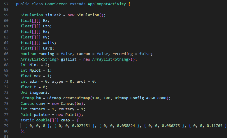
It remains the first and only Java code I’d ever written, and it shows – this was before ChatGPT, so I had to make do with as much copying and pasting as StackOverflow would allow. Phone processors were also much slower back then, and running numerical simulations was not something that they were used to doing.

It was time then to take those 1,089 lines of terrible Java, take stock, use all my might as a professional software engineer, and re-imagine them as 10,000 lines of terrible Typescript.

It’s glorious. Who needs more than one class anyway? Why would you write `canvas` when you could write `canv`?

Extracting the core

Fortunately, the core of the numerical algorithm to propagate WiFi waves is very simple, and I learnt about implementing the FDTD method from a book by Allen Taflove. In the simplest possible incarnation, you just need to update one vector component of the electric field, and 2 components of the magnetic field.

Here’s the electric field update step from the original app:

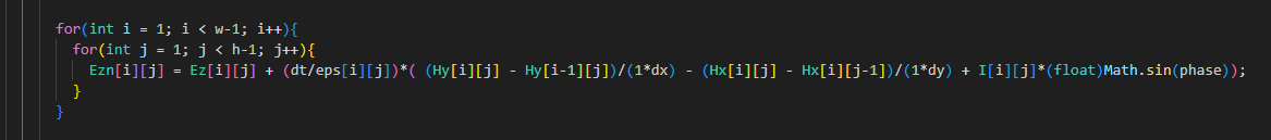
There’s a bit more to it than that, particularly around boundary conditions, but it’s really not rocket science – take some 2D arrays, and update them step-by-step. In total you’re dealing with less than 100 lines of code.

If you squint, you might also notice that the new electric field Ezn only depends on values from the previous step (i.e. there’s nothing on the right-hand-side with an n suffix). This means that the solver is trivially parallelisable – you can compute all of the new field values independently from the old ones.

Now, if you could get your hands on some kind of supercomputer with thousands of cores, maybe you could easily speed up this simulation by a huge amount…

Updating the solver

Fortunately these days we all carry massively powerful compute capabilities around with us – the CPUs in modern devices have gotten faster, but crucially so have the GPUs. In addition, modern APIs for performing computation on GPUs has also evolved – at time of writing, Chromium-based browsers can make use of the WebGPU API, and this will be coming soon to Safari and Firefox too.

Let’s take a look at the same code as above to compute a new electric field value, but written for a GPU:

It’s exactly the same! But with a crucial difference – the double for-loop around the computation has gone. This is because WebGPU allows you to write a compute shader which operates on a single element at a time, then parallelise that computation across all of the (potentially thousands) of cores on your GPU.

This speeds things up tremendously – you can run simulations at interactive speeds. Check out the video above for an example.

Updating the renderer

As the computation is now performed on the GPU, all of the data about the electromagnetic fields is also stored in GPU memory. This means it is sensible to render that data using the GPU too, which is done in 2 steps (if you’re interested, you should really check out WebGPU fundamentals):

Vertex shader – split up your scene into triangles, and figure out where those triangles should be
Fragment shader – colour in those triangles appropriately

The fragment shader was pretty simple – all we do is take a field amplitude, and map it against a colormap. In this case I took all of the popular ones I could find and jammed them in there. (You can go nuts on the homepage if you want to try some of them out!)

The vertex shader was more fun though – let’s step through how it works:

Step 1 – 2D

This step is very similar to the original app code – the field data is already laid out in a 2D array, so you just need to convert the field strength to a colour, and assign it to 6 vertices that define a small square:

Each element in the 2D array for the field strength becomes 2 triangles.

If you do this correctly, and colour in those triangles, you get a familiar heatmap-like image:

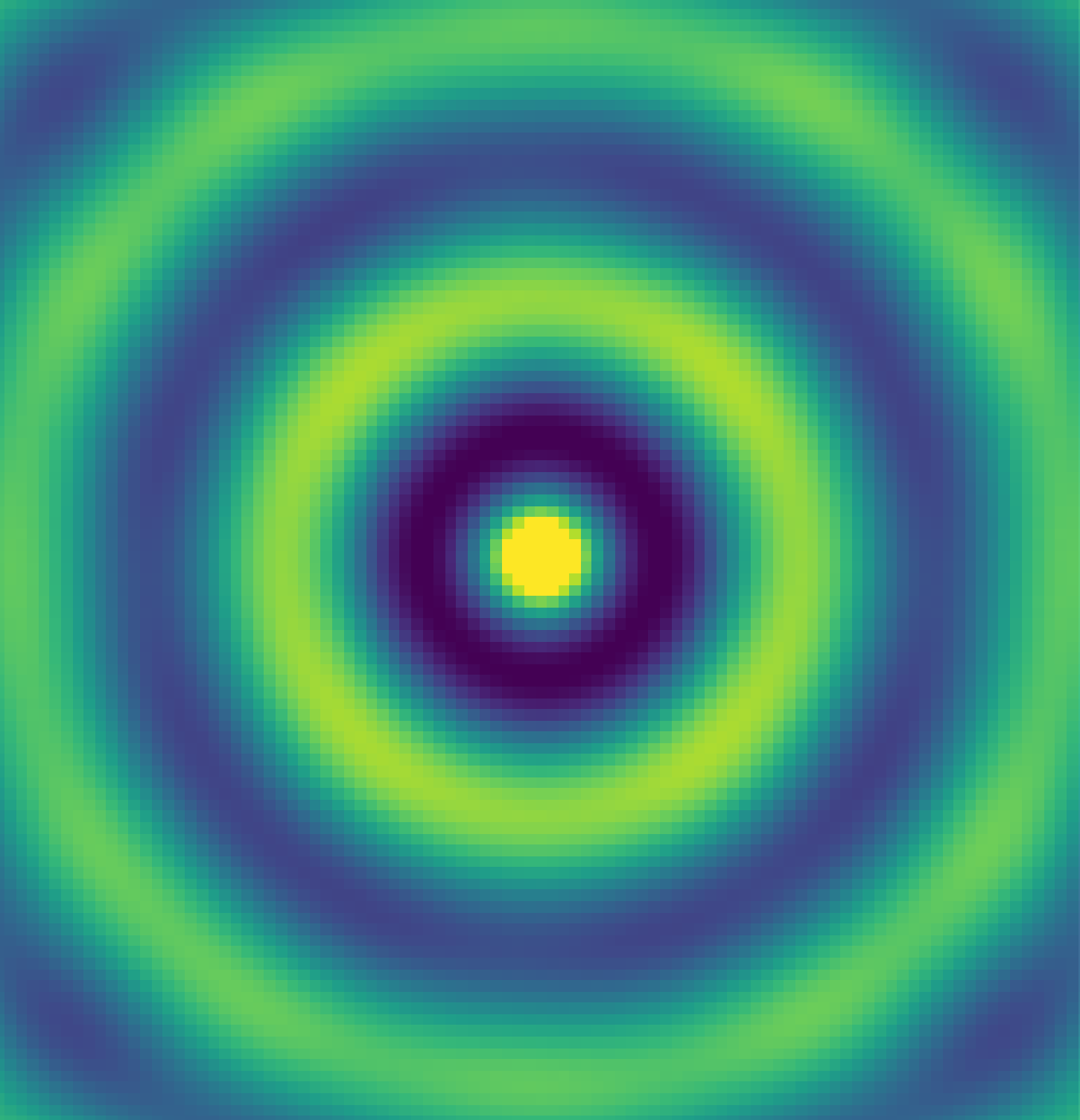
(In the real app, we don’t actually create this geometry for the 2D view, but instead use the fragment shader to colour in 2 large triangles.)

Step 2 – extend to 3D

This is also simple – just add some z offset proportional to the field strength:

Ah, perhaps it wasn’t that simple. Still, it’s not so difficult – as each square is made up of two triangles, we can bend the vertices of the square up and down to make sure they all join up:

This is looking great (and makes me wonder what on earth Matlab was doing most of the time – see here for some more Matlab ranting), but it does look a little flat.

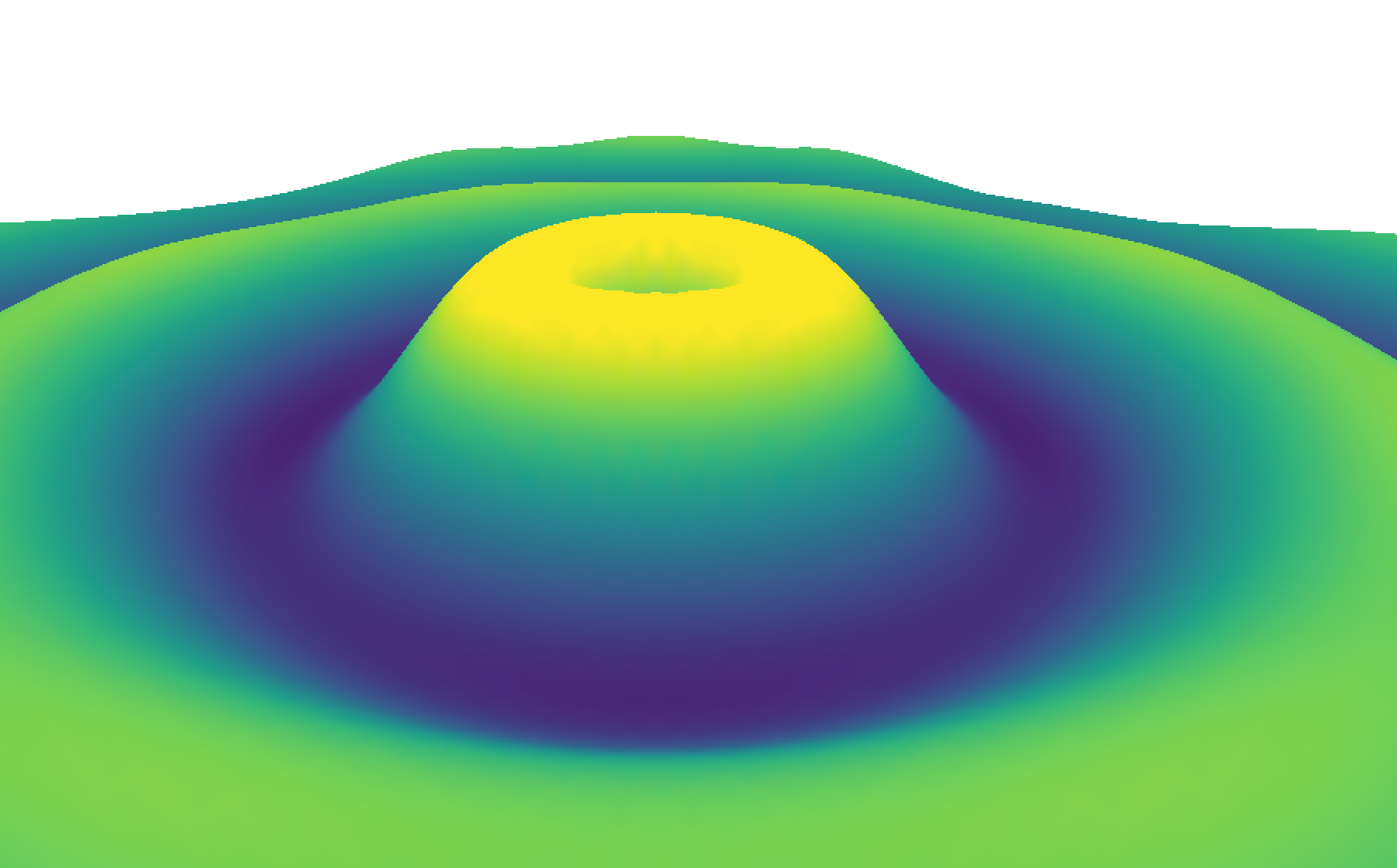
Step 3 – lighting

One of the other great uses of my time around writing the original app was learning Blender – there I learned the importance and mechanics of lighting.

The simple model we use here is to pick a single global sun direction $\mathbf{d}_{\text{sun}}$ , and mix in some sun colour to each triangle based on the orientation of the triangle. In particular, we compute the normal vector $\hat{\mathbf{n}}$ for each triangle and calculate the amount of sunlight to add as $\hat{\mathbf{n}} \cdot \mathbf{d}_{\text{sun}}$ :

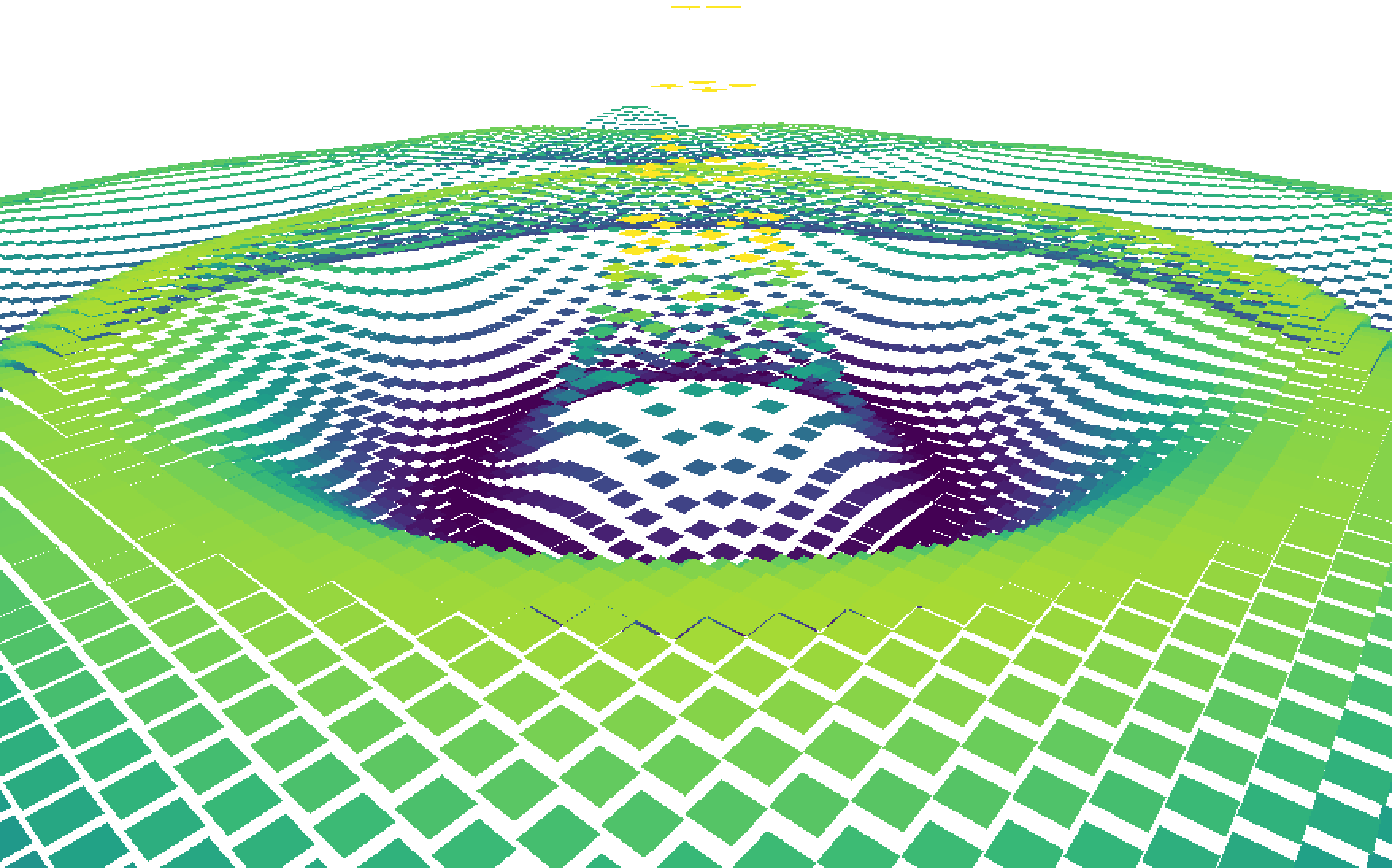
This lighting step does exactly what it says on the tin. Unfortunately, the tin said ‘make me look like a Playstation game from 1998’.

This is working exactly as intended though – each triangle does have a uniform normal vector across its surface, so the lighting is constant across the triangle. The harsh steps between triangles are due to the sudden change in normal vector, which is an artefact of the discretisation of the simulation grid.

We (and even Matlab for god’s sake) can do better though.

Step 4 – smooth normals

The final step in this rendering journey is to interpolate the normal vectors across the triangles of the mesh. This sounds complicated, but actually the GPU will help you here as it contains special hardware for interpolation. All we as shader writers have to do is define the appropriate values at each vertex, and interpolation across the triangle is automatic.

Consider the highlighted vertex below – it is surrounded by 6 triangles with slightly different normal vectors:

If you imagine sweeping the connected normals onto that vertex, then averaging them, you can define a normal vector for each vertex. If you then interpolate these vertex normals across the triangles, you get much smoother lighting:

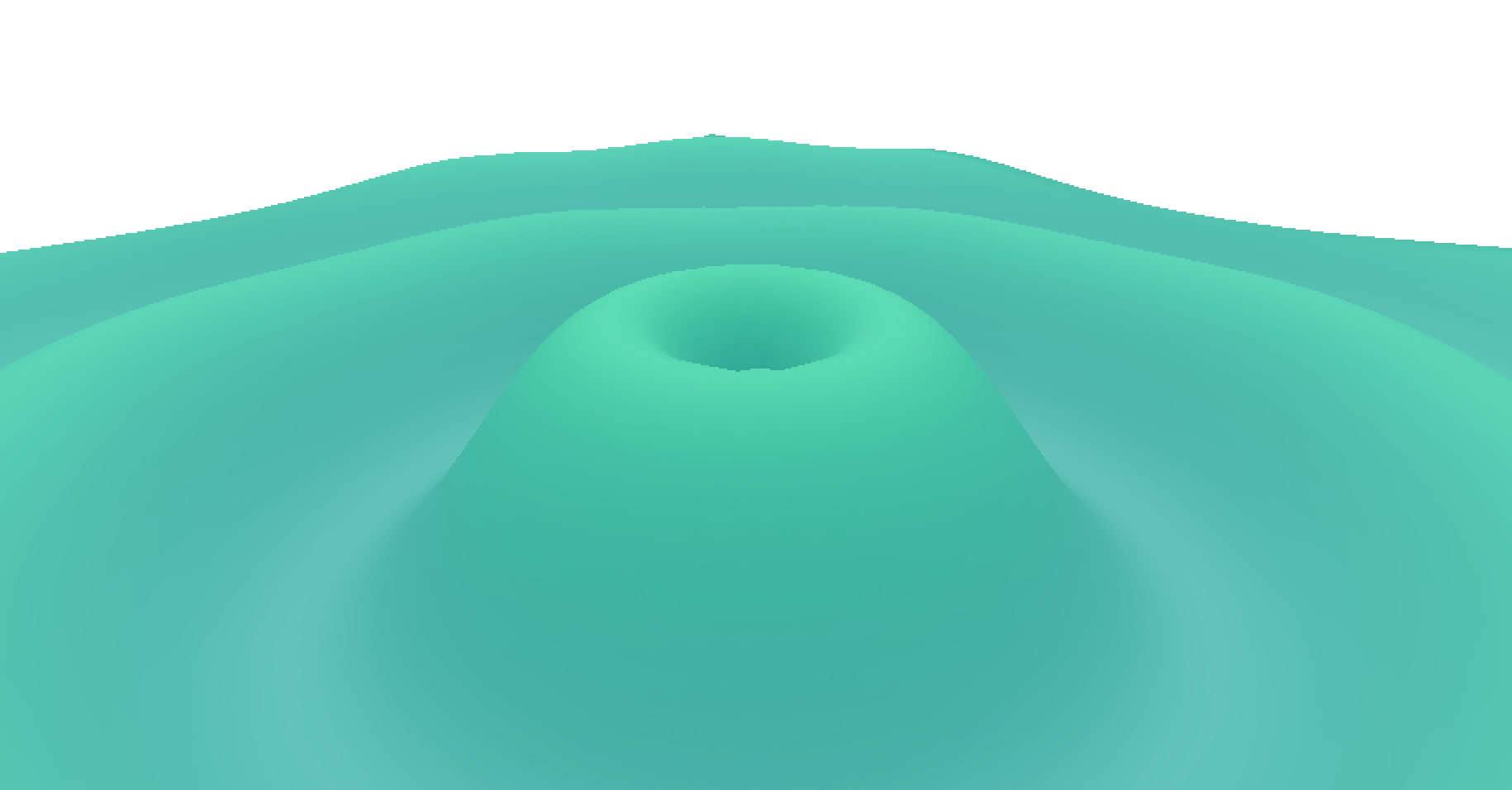
Now the textbooks don’t say this specifically, but you also get that ‘cool sciencey’ look too for free – a must for any serious data visualisation.

The stack

While there were still a few headaches remaining getting this simulation up and running in a web browser (particular shout-out to projection matrices and multi-touch), the rest of the app is much more standard – it’s written in Typescript, using React for rendering and Redux Toolkit for state management. All of the gnarly GPU stuff was written (badly) by yours truly, except for some matrix construction – here’s the package.json:

  "dependencies": {
    "@reduxjs/toolkit": "^2.2.3",
    "@types/react": "^18.2.52",
    "@types/react-dom": "^18.2.18",
    "@types/uuid": "^9.0.8",
    "@typescript-eslint/parser": "^7.0.2",
    "@webgpu/types": "^0.1.40",
    "firebase": "^10.9.0",
    "gl-matrix": "^3.4.3",
    "react": "^18.2.0",
    "react-dom": "^18.2.0",
    "react-redux": "^9.1.0",
    "react-router-dom": "^6.22.0",
    "styled-components": "^6.1.8",
    "uuid": "^9.0.1",
    "wgpu-matrix": "^2.5.1"
  },

The backend is also really simple – it’s almost all Cloudflare! Specifically:

The API ‘server’ is a Cloudflare Worker – small, ephemeral Typescript functions that receive a request and return a response.
The authentication uses Google Firebase.
The hosting and domain name is managed by Cloudflare.
The SQL database is Cloudflare D1, which seems to be a small wrapper around SQLite.
The image hosting is Cloudflare R2.
The payment processor is Stripe.
The documentation is hosted on Gitbook.

At the moment, I’m well within the free tier for all of these services. It’s pretty amazing how far you can get as a one-man band these days, and I’d definitely recommend checking these services out.

What next

It’s been a fun journey to write this new app – both nostalgic to read code I’d written in a mad korma-infused haze a decade ago – and instructive to approach the same problem again as a more seasoned software engineer.

It’s so darn easy to write updates too – just commit to GitHub, and Cloudflare builds and deploys a new version in a minute or so – so I’ll continue updating it. Some features I’m thinking about are:

Video export – ffmpeg in the browser perhaps?
Exporting raw simulation data – currently it’s all held on the GPU, but it would be nice to copy some of it back out again
AI simulations – Cloudflare has some AI features – would it be cool to take a simulation input and predict an output without running anything? Maybe, though that would number my days as a writer of numerical solvers…

If you read this far you’d probably enjoy it too – head over and look at some of the example sims. If you want access and can’t afford it, contact me and I’ll give you access anyway – I’m only trying to cover my hosting costs, which are currently zero. To the kind people that have already donated anyway – thank you!

While I don’t expect this new incarnation of WiFi Solver to affect my life as much as the first one did, I’m proud of it, and happy I managed to deliver an appropriate tribute (even if it meant I didn’t post for a year…). See you all in 2034!

PS – If you’re reading this and thinking ‘this Jason guy is pretty cool, I’d like to work with him’, maybe you can! Check out roles at my current company here.