Type IV radio emission is a broadband continuum, typically lasting minutes to hours, commonly attributed to energetic electrons trapped in coronal magnetic structures such as postflare arcades or coronal mass ejection (CME) flux ropes (A. Boischot 1957; J. P. Wild et al. 1963; M. Pick & N. Vilmer 2008; N. Gopalswamy 2011). In the hectometric band, only spacecraft can observe the emission because the terrestrial ionosphere is opaque below ∼10 MHz. Type IV bursts therefore provide a remote-sensing view of the changing corona and inner heliosphere, including particle acceleration, magnetic trapping, and the large-scale topology that couples the low corona to the solar wind (L. Klein et al. 1983). Both plasma emission near the fundamental/second harmonic of the plasma frequency and gyrosynchrotron emission have been invoked, with polarization often offering key constraints on the emission mode (D. B. Melrose 1980). In favorable cases, radio spectra and imaging allow estimates of magnetic field strength and source geometry.
Long-duration hectometric type IV bursts are rare. The longest previous example (2002 May 18–23) persisted for ∼5–6 days and showed strong circular polarization, hour-scale pulsations, and an apparent east-to-west drift consistent with a corotating source (M. J. Reiner et al. 2006). Notably, that episode was followed at Wind by an anomalously tenuous solar wind interval; Appendix C revisits the timing with radio and in situ data. A statistical survey likewise found only three events out of hundreds with durations ≳16 hr (A. Hillaris et al. 2016), and a Cycle 24 catalog reports typical hectometric type IV durations of tens of minutes to a few hours (A. Mohan et al. 2024). Many studies link type IV emission to CMEs and flux ropes, with longer events preferentially detected when the source lies within ∼60° of the Sun–observer line (H. M. Bain et al. 2014; N. Gopalswamy 2016).
At hectometric (f = 0.5–3 MHz) frequencies, the emission is often treated as plasma radiation near the plasma frequency (fundamental or harmonic). The electron plasma frequency is  MHz for ne cm−3, so fundamental emission in this band corresponds to ne ∼ 3 × 10³–1 × 105 cm−3. However, the near-unity circular polarization in some long-duration events, together with their association with unusually rarefied heliospheric intervals, also motivates considering electron-cyclotron maser emission (ECME) in low-density magnetic cavities where the plasma and cyclotron frequencies are comparable (R. M. Winglee & G. A. Dulk 1986a, 1986b). At these frequencies, ECME requires f ≃ fce = 2.8 B (MHz; B in G), i.e., B ∼ 0.18–1.1 G. For comparison, a radial r−2 field scaled from B ≈ 5–6 nT at 1 au implies B ∼ (2–5) × 10−2 G at r ∼ 6–10 R⊙ (our plasma-height range), so fce ≲ 0.06–0.14 MHz. In the fundamental plasma emission case (f ≃ fpe), our 0.5–3 MHz band implies fpe/fce ≈ 4–50 (about half these values for harmonic emission), i.e., typically ≳10 during the bright 1–2 MHz portion; ECME would then require either substantially enhanced B and/or a strong density depletion relative to the background. In that regime, the maser can preferentially excite X- or Z-mode waves; Z-mode (slow extraordinary) waves do not escape directly but could contribute via conversion at sharp density gradients. Recent in situ polarization analyses confirm that Langmuir/Z-mode waves are supported in the solar wind and that modest density fluctuations can account for their transverse polarization (T. Formánek et al. 2025), reinforcing the relevance of Z-mode physics for heliospheric radio sources.
Low-frequency solar radio waves are strongly affected by refraction and small-scale density inhomogeneities in the corona and solar wind, which deflect the apparent arrival direction and broaden the image of compact sources (J. L. Steinberg et al. 1984; E. P. Kontar et al. 2017, 2019; D. L. Clarkson et al. 2025). This propagation point-spread function explains why direction finding and image sizes at ≲10 MHz can greatly exceed intrinsic source scales and be only weakly frequency dependent over narrow bands (G. Thejappa et al. 2007; V. Krupar et al. 2018, 2020). Accounting for this scattering is essential both for localization and for size diagnostics. Imaging at higher frequencies (e.g., LOFAR) also shows height-frequency trends with source broadening consistent with scattering (M. Gordovskyy et al. 2022).
In this Letter, we report an exceptionally long hectometric type IV continuum observed over nearly 19 days in three successive visibility windows and seen in succession by Solar Orbiter, then in the Earth-facing hemisphere at Wind and Parker Solar Probe (overlapping in time), and finally at STEREO-A as the Sun rotates (Sections 2.1 and 2.2). The event links long-duration type IV emission to a corotating electron reservoir likely sustained by multiple CMEs and/or continued injection from the low corona. We leverage polarization and single-spacecraft direction finding, together with a wavevector-corrected ray sphere (WCRS) localization technique, to place the source near a helmet streamer (Sections 2.3 and 2.5) and to diagnose its size via quasiperiodic pulsations interpreted through magnetoseismology (Section 2.4). Section 3 synthesizes these results and discusses their broader implications.
2.1. Instrument Description
We use radio measurements from Solar Orbiter, Wind, Parker Solar Probe, and STEREO-A, which together provide complementary longitudes and heliocentric distances. The Radio and Plasma Waves (RPW) instrument on Solar Orbiter (D. Müller et al. 2013; M. Maksimovic et al. 2020) records spectral power with the Thermal Noise Receiver (TNR; 2 kHz–1 MHz) and the High Frequency Receiver (HFR; 375 kHz–16 MHz). Level-2 V2 Hz−1 spectra are converted to solar flux units (sfu; 1 sfu = 10−22 W m−2 Hz−1) and normalized to a 1 au distance using a 1/r2 profile, with the calibration summarized in Appendix A.
The WAVES instrument on Wind (J.-L. Bougeret et al. 1995; L. B. Wilson et al. 2021) provides RAD1 (20–1040 kHz) and RAD2 (1075 kHz–13 MHz) spectra. We convert V2 Hz−1 to sfu with the instrument responses (Appendix A). For this event, Wind direction finding was not used because the available calibrated RAD1 product assumes an unpolarized source, whereas our event is strongly polarized.
Parker Solar Probe carries the FIELDS suite (S. D. Bale et al. 2016; N. J. Fox et al. 2016), which includes a radio-frequency receiver providing low-frequency spectra and polarization. We use Parker Solar Probe/FIELDS flux and degree of circular polarization V/I measurements in the 0.5–3 MHz band during 2025 September 4 00:00–September 6 14:00 (Figures 1(c), (d)), when Parker Solar Probe was at ∼0.4 au, to complement Wind and to provide an additional polarization constraint at a smaller heliocentric distance.
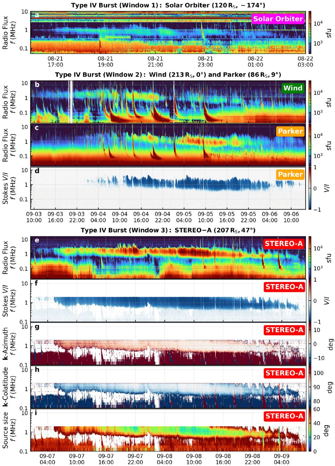
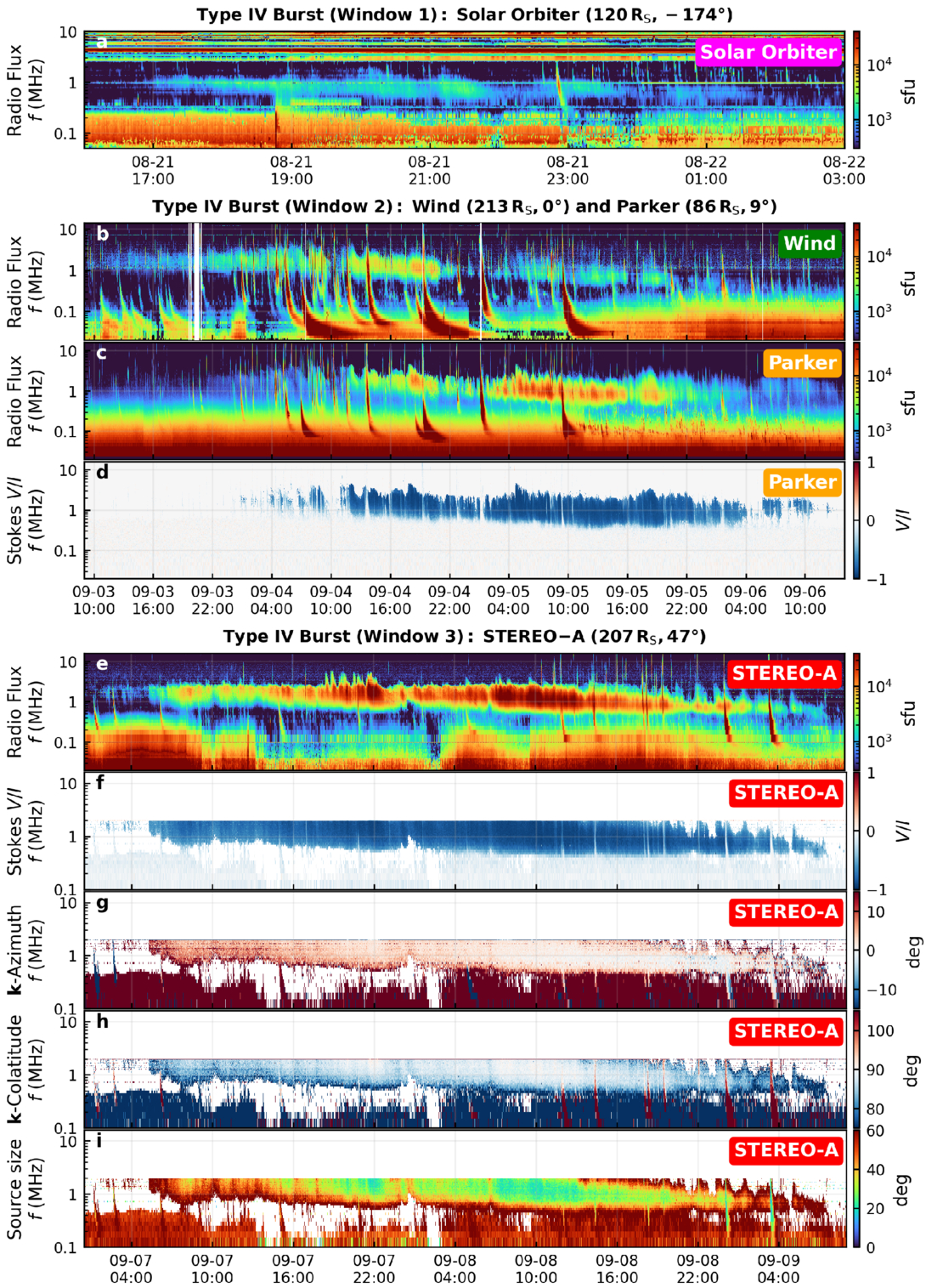
Figure 1. Event overview of the 19 day corotating type IV continuum. (a) Solar Orbiter/RPW dynamic spectrum (Window 1). (b) Wind/WAVES and (c) Parker Solar Probe/FIELDS flux (Window 2; Wind-Parker Solar Probe overlap). (d) Parker Solar Probe circular polarization V/I (negative values correspond to left-hand circular polarization). (e) STEREO-A/WAVES flux (Window 3). (f) STEREO-A circular polarization V/I. (g)–(i) STEREO-A wavevector azimuth, colatitude, and apparent source size. The apparent cutoff at 2 MHz reflects the direction-finding data product limitation.
Download figure:
Standard image High-resolution imageThe STEREO/WAVES experiment on STEREO-A (J. L. Bougeret et al. 2008; M. L. Kaiser et al. 2008) measures radio power, polarization, and wavevector direction with a triad of monopole antennas. We use Level-3 data (already in physical units of sfu) from 125 kHz to 2 MHz, which provide Stokes I, V, the wavevector direction (azimuth and colatitude in RTN), and an apparent source size γ at STEREO-A (V. Krupar et al. 2022). Direction-finding products are available only up to 2 MHz; consequently, the STEREO-A polarization and direction-finding panels in Figure 1 show an apparent upper-frequency cutoff at 2 MHz.
2.2. Event Overview
From 2025 August 21 to September 9, a single long-lived type IV continuum was detected in three successive visibility windows by four spacecraft as solar rotation carried the source region from the farside into the Earth-facing hemisphere and onward toward STEREO-A longitudes. We refer to these three intervals as Windows 1–3 (Figure 1); they represent observer-dependent visibility of the same corotating reservoir rather than three independent bursts.
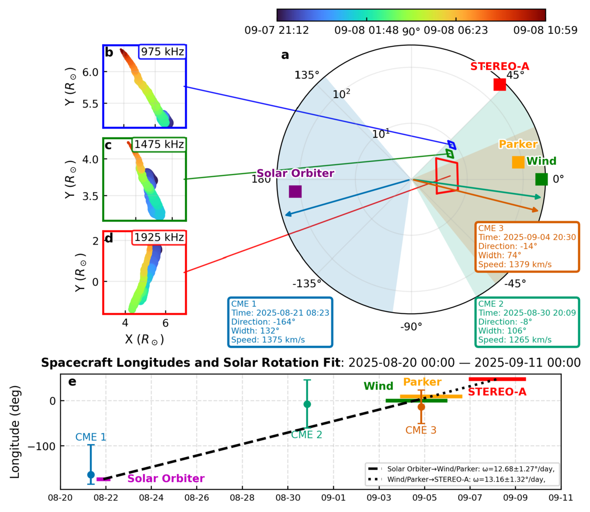
The observing geometry is summarized in Figure 2. The spacecraft heliocentric distances and heliolongitudes during the three windows (given above each panel in Figure 1) were Solar Orbiter at 120 R⊙ and λ ≈ −174° (Window 1), Wind at 213 R⊙ and λ ≈ 0° and Parker Solar Probe at 86 R⊙ and λ ≈ 9° (Window 2), and STEREO-A at 207 R⊙ and λ ≈ 47° (Window 3). The horizontal bars in Figure 2(e) indicate these visibility windows in longitude-time space, while the polar view in Figure 2(a) places the observers relative to the CME propagation wedges. A linear fit to the window centroids yields synodic rotation rates ω = 12 68 ± 1
 27 day−1 (SolO → Wind/Parker Solar Probe) and ω = 13
 16 ± 1
 32 day−1 (Wind/Parker Solar Probe → STEREO-A), corresponding to periods P ≈ 28.38 ± 2.84 and 27.35 ± 2.74 days (Figure 2(e)).
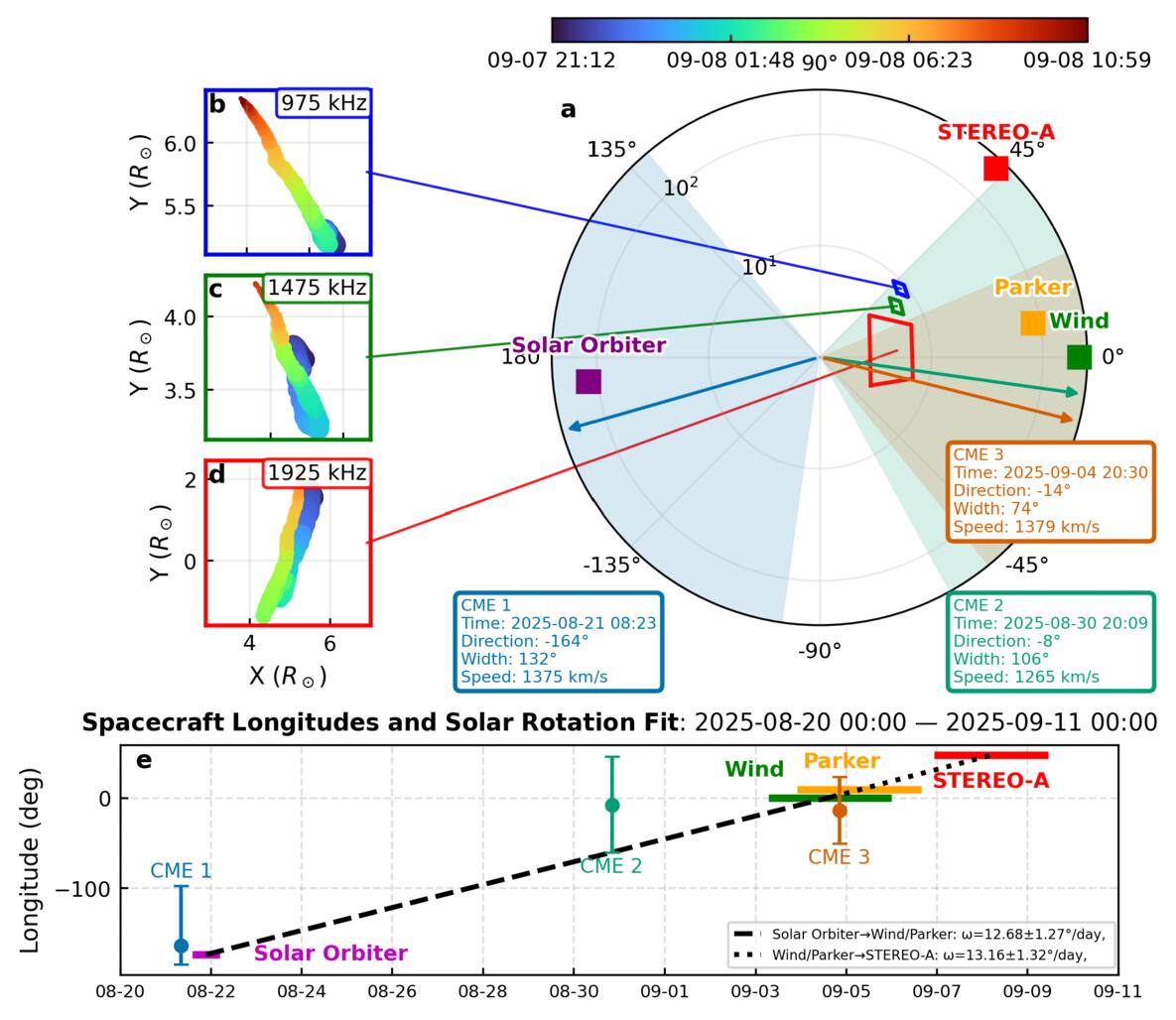
Figure 2. WCRS localization and observing geometry. (a) Polar view with spacecraft positions (red filled square: STEREO-A; green: Wind/Earth; orange: Parker Solar Probe; purple: Solar Orbiter); the radial coordinate is logarithmic. Colored wedges indicate the propagation directions and full angular widths of three fast CMEs, with onset times and sheath (shock-front) speeds from the NASA/CCMC DONKI CME catalog (coronagraph-based fits from available viewpoints). We use these catalog fits for timing/geometry context only; uncertainties are larger for the farside CME1, and we do not attempt a detailed CME reconstruction. (b)–(d) WCRS source trajectories (close-side ray-sphere solutions) for 975, 1475, and 1925 kHz, projected onto the HEEQ equatorial (x–y) plane and color coded by time during Window 3. (e) Spacecraft heliolongitudes vs. time; horizontal bars mark the three type IV visibility windows.
Download figure:
Standard image High-resolution imageFigure 1(a) shows Window 1: a weak continuum around 1 MHz on 2025 August 21 16:00–August 22 03:00 detected by Solar Orbiter at ∼0.6 au while the source region was on the farside as viewed from Earth. Despite spacecraft electromagnetic disturbances (M. Maksimovic et al. 2021), the spectra reveal a broad continuum characteristic of interplanetary type IV emission.
Twelve days later, as the source rotated into a more favorable geometry, the continuum intensified and persisted much longer. Window 2 was observed near Earth by Wind on 2025 September 3 09:00–September 5 22:00 (Figure 1(b)). Parker Solar Probe observed the same continuum on 2025 September 4 00:00–September 6 14:00 (Figure 1(c)) with concurrent circular polarization V/I measurements (Figure 1(d), negative values correspond to left-hand circular polarization), overlapping the Wind interval and confirming continuity of the corotating reservoir. Wind and Parker Solar Probe also observed enhanced type III activity in the days surrounding CME2 (2025 August 30), including a pronounced type III storm and complex type III bursts (Figures 3(c),(d)). This storm-like activity suggests sustained electron injections onto open magnetic field lines during CME-driven magnetic reconfiguration.

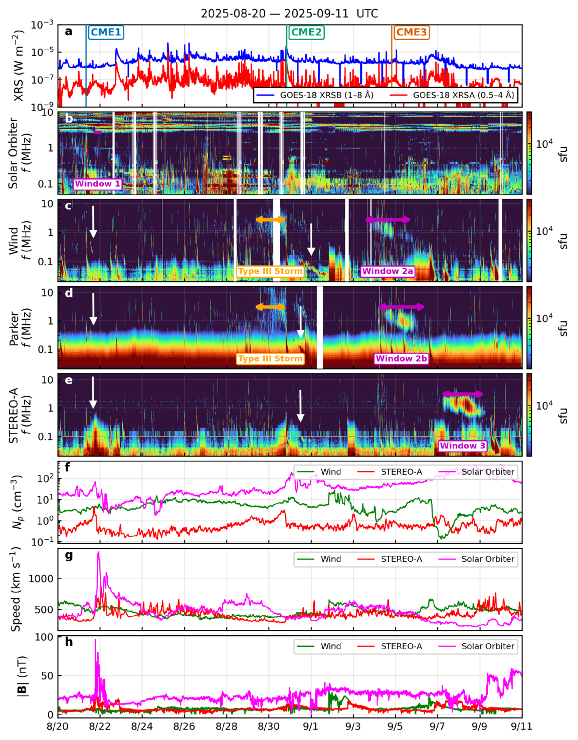
Figure 3. Overview of flare, radio, and in situ context for the long-duration type IV event. (a) GOES-18 X-ray flux (1–8 Å). Because GOES is an Earth-view proxy, panel (a) may not capture farside activity during Window 1/CME1. (b)–(e) Radio dynamic spectra from four spacecraft: (b) Solar Orbiter/RPW, (c) Wind/WAVES, (d) Parker Solar Probe/FIELDS, and (e) STEREO-A/WAVES. (f)–(h) In situ solar wind parameters measured at Wind (green) and STEREO-A (red): (f) Proton density np, (g) bulk speed VSW, and (h) magnetic field strength ∣B∣. Solar Orbiter (magenta) is also shown for np and VSW. Vertical lines in panel (a) indicate the launch times of the three fast CMEs, color coded as in Figure 2 (times from DONKI; see the text). The white arrows in panels (c)–(e) indicate type II bursts.
Download figure:
Standard image High-resolution imageOne day later, Window 3 was observed by STEREO-A on 2025 September 7 00:30–September 9 09:00 (Figure 1(e)); at that time STEREO-A was located ∼47° ahead of Earth in heliolongitude. The corresponding V/I (Figure 1(f)) is predominantly negative (nearly pure left-hand circular polarization), indicating that the continuum is dominated by a single magnetoionic mode.
Figures 1(g) and 1(h) show the STEREO-A wavevector direction  in the RTN frame (
 from the Sun to the spacecraft,
  prograde in the orbital plane, and
  ). The azimuth decreases steadily from eastward (positive) toward ≈0°, consistent with slow rotation-parallax drift, while the colatitude remains slightly <90°, indicating a modest southward offset. Finally, Figure 1(i) shows the apparent source size γ, which varies between ∼20° and ∼40°, with smaller sizes coincident with the brightest intervals.
We also note a systematic downward drift of the continuum’s characteristic frequency and a gradual narrowing of its bandwidth over each visibility window. In Window 3, the bright ridge shifts from ∼1 to 2 MHz near the start toward ∼0.5–1 MHz near the end. A similar drift is apparent in the Wind and Parker Solar Probe spectra during Window 2. Because this trend is observed from multiple heliolongitudes, it is unlikely to arise solely from a single structure propagating radially through the solar wind; instead, it may reflect corotation and changing visibility of different portions of a large loop/streamer-top trap as the system rotates.
The sequential appearance of the continuum at the three vantage points, with delays consistent with solar rotation, suggests a fixed source region that becomes detectable only within an effective longitudinal visibility window (a lighthouse effect). During the strong phase, the visibility durations are 61 hr at Wind, 62 hr at Parker Solar Probe, and 56.5 hr at STEREO-A (Window 2 and Window 3; Figure 1). For a corotating source, these durations imply an effective detectability width Wvis ≈ Ω⊙Tvis ≃ 31°–34° (full width) for Ω⊙ ≈ 13 2 day−1 (consistent with the rotation rates inferred from the window-to-window handoffs). An independent constraint comes from the rapid Parker Solar Probe → STEREO-A handoff: the continuum ends at Parker Solar Probe on 2025 September 6 14:00 and begins at STEREO-A on 2025 September 7 00:30, while the spacecraft longitudes differ by Δλ ≃ 38° (Parker Solar Probe at λ ≈ 9°, STEREO-A at λ ≈ 47°; Figure 2(e)). The 10.5 hr gap corresponds to only Ω⊙Δt ≈ 6° of solar rotation with no detection at either spacecraft; interpreting this as a blind longitudinal sector implies Wvis ≈ Δλ − Ω⊙Δt ≈ 32° (about ±16° about central meridian). We stress that Wvis is an effective detectability window shaped by intrinsic anisotropy, occultation by dense coronal/CME structures, and propagation effects (refraction/scattering) at hectometric frequencies, rather than a literal narrow emission beam. Consequently, nondetections between the windows should not be interpreted as cessation of the reservoir; the emission can persist but fall below detectability outside the visibility window. In Section 2.3, we therefore use the more restrictive, high-confidence duration within Window 3 to estimate the geometric transverse diameter Wrot of the emitting trap, while Wvis should be regarded as an effective detectability width (upper limit).
Three fast CMEs erupted during the interval—CME1 on 2025 August 21, CME2 on August 30, and CME3 on September 4—with sheath (shock-front) speeds of ≈1375, ≈1265, and ≈1379 km s−1, respectively (propagation directions and angular widths summarized in Figure 2).10 CME1 and CME2 were accompanied by hectometric type II radio emission; for CME2, the associated interplanetary shock was also sampled in situ near Earth by Wind. CME3 was followed by an unusually low solar wind proton density at Wind, np ∼ 0.1 cm−3 (the absolute value at such low densities may carry increased uncertainty, but the rarefaction itself is robust). Each of the three CMEs appears to correspond to an enhancement or continuation of the type IV burst.
We present additional observations and context for the long-duration type IV radio burst event. Figure 3(a) shows the Earth-view GOES-18 soft X-ray flux (1–8 Å and 0.5–4 Å) for context. Several moderate enhancements are visible near CME2 and CME3. Because CME1 originated on the farside of the Sun, any associated soft X-ray emission may be poorly represented in GOES; complementary farside diagnostics (e.g., Solar Orbiter/STIX) are beyond the scope of this work. Figures 3(b)–(e) compile the multispacecraft dynamic spectra and mark Windows 1–3 (magenta arrows) discussed in Section 2.2, together with flare/CME and in situ context. A pronounced type III storm is visible around CME2 (2025 August 30; orange arrow in Figures 3(c),(d)), together with complex type III activity (J. Zhang et al. 2024; M. Pulupa et al. 2025). This storm precedes the Wind/Parker Solar Probe type IV visibility Window 2 (magenta arrows) rather than immediately preceding the type IV onset. Such storm-like activity implies sustained access of the source region to open field lines and ongoing reconnection; its timing near CME2 is consistent with CME-driven magnetic field reconfiguration that intermittently modifies open field connectivity and hence the type III burst rate.
Figures 3(f)–(h) show in situ solar wind measurements from Wind (green curves), Solar Orbiter (magenta; where available), and STEREO-A (red curves) over the course of the event. Figure 3(f) gives the proton number density (np), Figure 3(g) the bulk solar wind speed (VSW), and Figure 3(h) the total magnetic field strength (∣B∣). Several effects of the fast CMEs are evident in the near-Earth data (Wind, green).
CME1, which erupted on 2025 August 21, originated from a farside active region; it was associated with a hectometric type II radio burst (consistent with a CME-driven shock).
CME2, launched on 2025 August 30, drove a global shock that not only produced a type II burst but was also detected in situ: at Wind around September 1–2, the proton density and magnetic field show abrupt jumps, and the solar wind speed surges, signatures of the interplanetary shock.
CME3, erupting on 2025 September 4, did not have an obvious type II radio signature, but its passage had a dramatic impact on the solar wind: Wind observed an extremely low-density plasma void (with np dropping to ∼0.1 cm−3) in the days after the eruption. This rarefied interval, evident in Figure 3(f), suggests that CME3 over-expanded and generated an exceptionally rarefied trailing wake, leading to a transient “disappearance” event in the solar wind density. Similar low-density anomalies have been observed in the wake of some fast CMEs. The STEREO-A in situ measurements (red curves) show corresponding solar wind conditions from its vantage point, though the CME impacts at STEREO-A were less pronounced. Notably, STEREO-A did not experience as deep a density drop after CME3, consistent with the possibility that the bulk of CME3’s rarefied wake was directed toward Earth’s longitude. Such rarefied wakes may also enhance hectometric radio visibility by reducing propagation blurring along the line of sight, as suggested for the 2002 May long-duration type IV event ( Appendix C).
These contextual data confirm the temporal relationship between the CME eruptions and the observed radio and in situ signatures: CME1 and CME2 coincided with intense radio bursts (types II and IV), while CME3’s aftermath is captured by the anomalous drop in solar wind density.
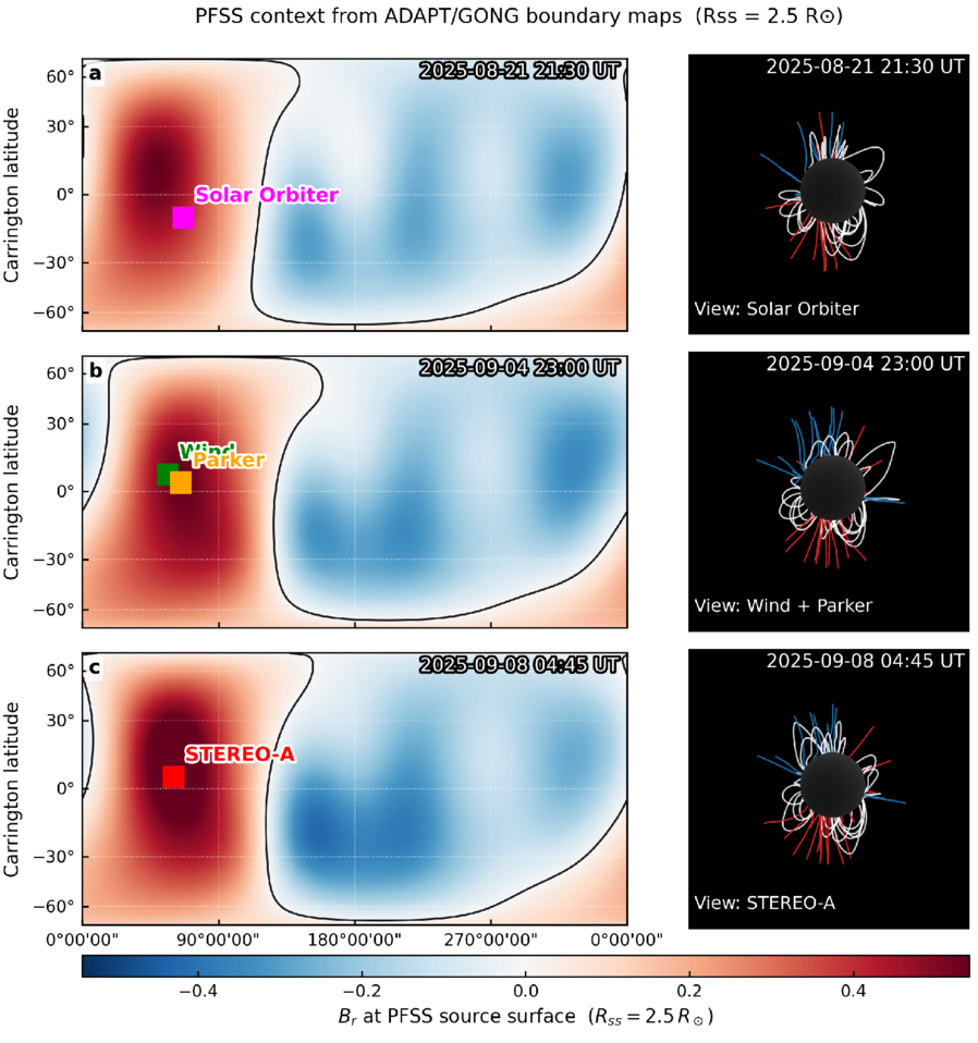
Figure 4 provides a potential field source surface (PFSS) context for the three representative epochs used in this work (M. D. Altschuler & G. Newkirk 1969; K. H. Schatten et al. 1969; J. Worden & J. Harvey 2000; P. Riley et al. 2006). The PFSS extrapolations were computed from ADAPT photospheric boundary maps assimilating NSO/GONG synoptic magnetograms (J. W. Harvey et al. 1996; C. N. Arge et al. 2010; K. S. Hickmann et al. 2015). The source-surface polarity inversion line (PIL) outlines the streamer belt/heliospheric current sheet footprint at Rss = 2.5 R⊙. The observing spacecraft samples a similar Carrington sector relative to this PIL as the Sun rotates, supporting the interpretation that the long-duration hectometric continuum is associated with a long-lived, corotating large-scale structure rooted near the streamer belt. Notably, the projected observer locations in all three windows fall on the Br > 0 side of the source-surface PIL. Moreover, in each window, the nearest segment of the source-surface PIL lies roughly ∼90° eastward of the projected sub-spacecraft longitude, placing the streamer belt near the corresponding east limb in each spacecraft’s view; this is consistent with the PFSS renderings (right panels of Figure 4) and with the streamer-like white-light context during Window 3, discussed later in Section 2.5. If the hectometric ray path remains predominantly in this magnetic sector out to 1 au, the observed persistent left-hand circular polarization at STEREO-A is consistent with ordinary-mode (O-mode) emission (Section 2.3). We emphasize that PFSS is used here only for global topological context; above Rss, the model field is forced radial and therefore cannot be used to infer detailed magnetic geometry or mode-coupling effects at the hectometric source heights.
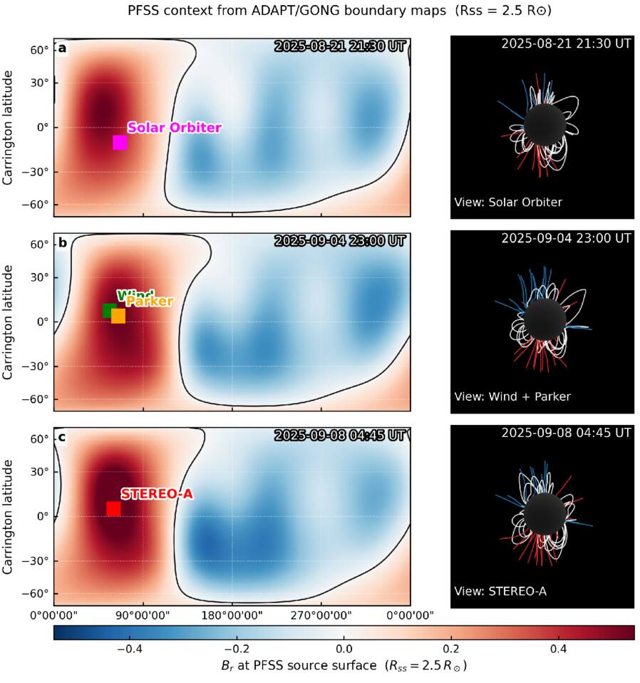
Figure 4. PFSS context for the long-duration type IV event, computed from ADAPT/GONG boundary maps with source-surface radius Rss = 2.5 R⊙. Left panels: radial magnetic field Br at the PFSS source surface (red: Br > 0, blue: Br < 0); the source-surface PIL is shown in black. Squares mark the Carrington longitude/latitude of each observing spacecraft projected onto the source surface at representative times in the three visibility windows: (a) Solar Orbiter (2025 August 21 21:30 UT), (b) Wind and Parker Solar Probe (2025 September 4 23:00 UT), and (c) STEREO-A (2025 September 8 04:45 UT). Right panels: PFSS field lines traced from r = 1.2 R⊙ and rendered from the corresponding spacecraft viewpoint; closed field lines are white and open field lines are colored by polarity (red: Br > 0, blue: Br < 0). The PIL is located roughly ∼90° eastward of each projected spacecraft longitude at these epochs, suggesting that the relevant helmet streamer lies near the visible east limb from each viewpoint.
Download figure:
Standard image High-resolution image2.3. STEREO-A Direction Finding and Polarization
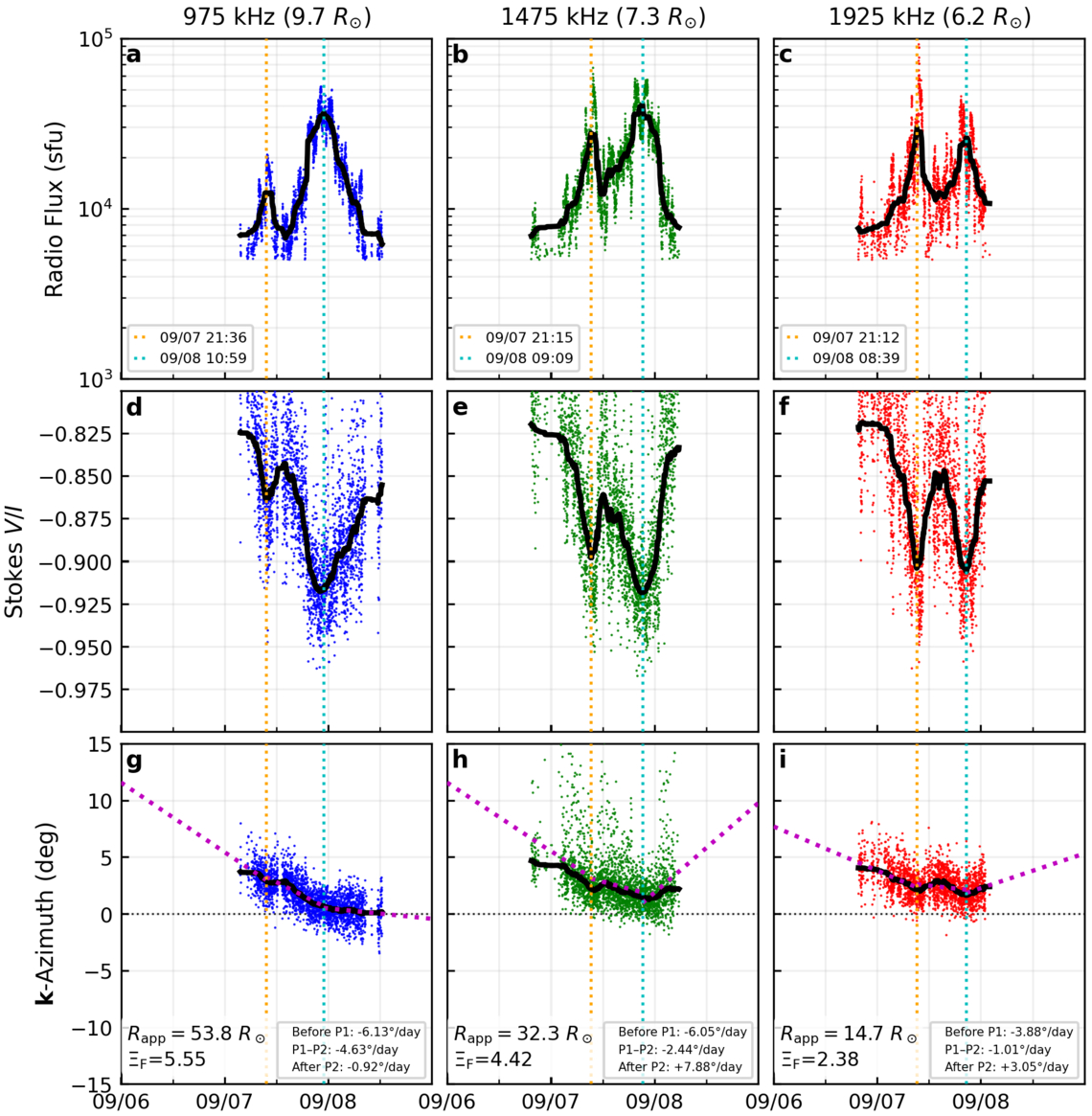
STEREO-A provides the most complete diagnostics during the brightest phase of the event. The geometry used below to relate the rotation duration and direction-finding angles to the physical source size and the WCRS correction is summarized in Figure 5. Figure 6 shows the time series at three representative frequencies (975, 1475, and 1925 kHz). The top row presents Stokes I (sfu) with a smoothed trend; the middle row shows the circular polarization V/I; the bottom row shows wavevector azimuth. We select high-confidence measurements with I > 5 × 10³ sfu and V/I < −0.8 to avoid weak, noisy intervals.
We estimate the source’s transverse size from the emission’s duration at STEREO-A combined with the Sun’s rotation. Durations after thresholding are T = {34, 35, 32} hr for 975, 1475, and 1925 kHz. These durations correspond to the high-confidence, strongly polarized portion of Window 3 (Figure 6); using the full Window 3 visibility duration (56.5 hr; Section 2.2) would yield a larger effective width and is best treated as an upper limit because detectability can also be shaped by beaming and propagation. With synodic rotation Ω⊙ = 13 2 day−1 and modeled radii r = {9.7, 7.3, 6.2} R⊙ (E. C. Sittler & M. Guhathakurta 1999), the rotation-to-size conversion is

yielding Wrot,975 = (3.15 ± 0.95) R⊙, Wrot,1475 = (2.44 ± 0.73) R⊙, and Wrot,1925 = (1.90 ± 0.57) R⊙ (1σ; dominated by a 30% height-mapping systematic). The band-averaged size is 〈Wrot〉 = (2.50 ± 0.75) R⊙. The rotation-duration geometry used to convert T into a transverse size Wrot is sketched in Figure 5(a). This is the chord length subtending the rotation angle Δϕ = Ω⊙T/24 at radius r, hence  (and Wrot ≈ r Δϕ for Δϕ ≪ 1 in radians).
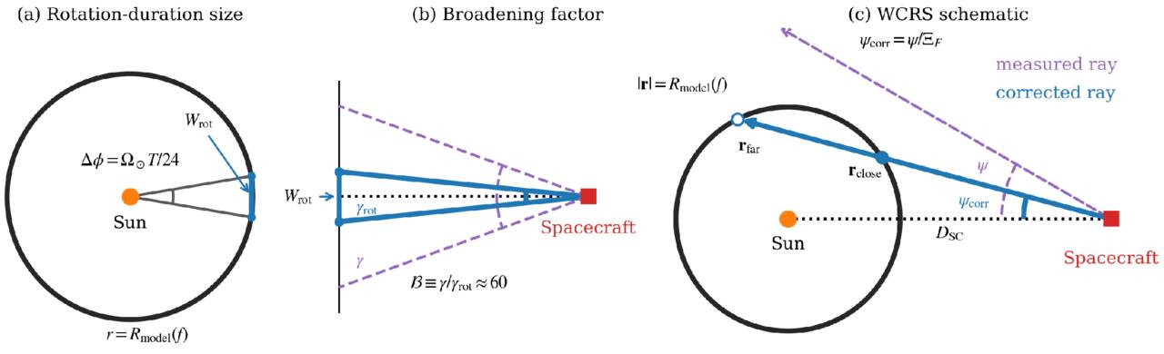
Figure 5. Geometry to relate rotation durations and direction-finding angles to a physical source size and to the WCRS correction. (a) A corotating source at heliocentric radius r = Rmodel(f) rotates through Δϕ = Ω⊙T/24 during an interval of duration T (in hours), corresponding to a transverse chord length  . (b) The same chord subtends a geometric angular half-width γrot at the spacecraft (Sun–spacecraft distance DSC); comparing with the goniopolarimetric apparent half-width γ defines the angular-broadening factor
  . (c) Schematic of the WCRS construction: the measured direction finding ray (dashed purple) has an angular deviation ψ from the Sun–spacecraft line; applying the scattering correction shrinks the deviation to ψcorr = ψ/ΞF (solid blue). Intersecting the corrected ray with the density model sphere ∣r∣ = Rmodel(f) yields the near- and farside solutions rclose and rfar.
Download figure:
Standard image High-resolution imageWe use W for the physical full transverse diameter of the emitting trap (half-width a ≡ W/2). Two independent estimators of the same W are used: Wrot from rotation geometry (Equation 1) and  from quasiperiodic pulsations (Section 2.4). When comparing to models that write the period as P ∝ L/vA, L denotes a characteristic length scale of the oscillating structure; the appropriate geometric factor depends on the specific eigenmode (see Section 2.4, Equation 3).
We denote the goniopolarimetric apparent half-width at the spacecraft by γ and the rotation-based geometric half-width by γrot. Here, B ≡ γ/γrot denotes the angular-broadening factor and is distinct from the magnetic field model Bcor(r) used later in the Alfvén speed estimate (Figure 5(b)). At DSC = 207 R⊙ (the Sun–spacecraft distance during Window 3), the above Wrot correspond to γrot = {0 44 ± 0
 13, 0
13, 0 34 ± 0
 10, 0
10, 0 26 ± 0
 08}. Here, γrot is the geometric angular half-width subtended by the corotation chord at the spacecraft (i.e., for small angles, γrot ≈ Wrot/(2DSC)). With γ ≃ 20° in all three bands, the apparent-to-geometric factors are
  ;
;  , 59 ± 18, and 76 ± 23 for 975, 1475, and 1925 kHz, respectively; combining the bands we adopt
  (1σ; systematic dominated; Figure 5(b)).
For context, the modeled source heights span Δr ≈ 3.5 R⊙ across the band, comparable to the band-averaged transverse diameter 〈Wrot〉 = (2.50 ± 0.75) R⊙. These radii are obtained from the E. C. Sittler & M. Guhathakurta (1999) density model under the fundamental plasma emission assumption used for the numerical estimates in this work. We defer the physical interpretation of both Δr and the large broadening factor  to Sections 3.2 and 3.5. This comparable radial and transverse extent suggests a large, streamer-top/flux-rope scale trap (i.e., a large closed coronal structure near the helmet streamer cusp and/or a CME flux-rope cavity) whose transverse and radial dimensions are of the same order at these heights.
The very large  points to strong angular broadening—plausibly multipath scattering by solar wind density inhomogeneities—while the near-constant γ across 1–2 MHz hints that propagation effects, rather than intrinsic source expansion, dominate the observed apparent size in this instance.
Direction-finding products are not available for Solar Orbiter and Parker Solar Probe, and we do not use Wind/WAVES direction finding because the available calibrated RAD1 direction-finding product assumes an unpolarized source (Section 2.1). However, Wind observed a comparably long type IV interval (over 2 days), suggesting a similar source size was present from Earth’s viewpoint. In contrast, Solar Orbiter saw only a much shorter continuum burst.
Two broad intensity maxima are evident at each frequency (vertical markers P1 and P2). For 975 kHz, P1 and P2 occur near 2025 September 7 21:36 and September 8 10:59; for 1475 kHz at 21:15 and 09:09; and for 1925 kHz at 21:12 and 08:39. From the offsets between the 1.925 and 0.975 MHz peak times, the P1 envelope implies an apparent pattern speed of ∼1600 km s−1 across the modeled height range—comparable to the CME speeds listed in Figure 2(a) and plausibly reflecting the passage of the CME-driven disturbance across the relevant density shells (E. C. Sittler & M. Guhathakurta1999). By contrast, the P2 offsets imply ∼280 km s−1, suggestive of a slower reconfiguration (e.g., expansion of the post-CME cavity or sheath, rotation-parallax-modulated visibility, or a low-phase-speed MHD disturbance within the trap); we therefore treat this second value as indicative rather than a direct measure of a propagating front. The uncertainty is dominated by peak-time selection and the adopted density–height mapping (E. C. Sittler & M. Guhathakurta 1999).
For the STEREO/WAVES polarization product used below, negative V/I denotes left-hand circular polarization in the adopted Level-3 sign convention. Any magnetoionic mode inference in this Letter is therefore referenced to that convention and should be regarded as conditional on it. Stokes V remains negative throughout, with ∣V/I∣ ≳ 0.9 near the peaks, indicating nearly pure left-hand circular polarization in the STEREO/WAVES sign convention. In the magnetoionic framework, such near-unity V/I suggests emission dominated by a single mode; for plasma emission at (or near) the fundamental frequency, the escaping mode is often expected to be the ordinary (O) mode (D. B. Melrose 1980; D. J. McLean & N. R. Labrum 1985). The PFSS sector context (Figure 4) indicates that the relevant lines of sight lie on the Br > 0 side of the source-surface PIL, suggesting that the observed left-hand sense could be compatible with O-mode emission under standard quasi-longitudinal assumptions. This mode inference, however, depends on the adopted Stokes-V convention and could be modified by mode coupling (e.g., quasi-transverse layers) or heliospheric current sheet/sector crossings along the ray path.
We measure the azimuth ϕ(t) of the incoming wavevector  in the spacecraft RTN frame. Even if the source corotates at fixed Carrington longitude, a finite heliocentric distance r produces a slow parallax sweep of ϕ(t) as the Sun turns; only r → 0 would keep ϕ constant. This rotation-parallax effect has long been used to infer interplanetary source distances from the drift of the apparent direction (J.-L. Bougeret et al. 1984).
Between P1 and P2 the azimuth drifts steadily (negative denotes west-to-east motion): −4.63, −2.44, and −1.01 deg day−1 at 975, 1475, and 1925 kHz, respectively (Figures 6(g)–(i)). Under the corotation hypothesis, this drift provides a purely geometric constraint on the apparent rotation radius,
where DSC is the Sun–spacecraft distance and Ω⊙ is the synodic rotation rate as seen from DSC (we adopt 13.2 deg day−1 at 1 au). Using DSC ≈ 207 R⊙ yields Rapp ≈ 53.8, 32.3, and 14.7 R⊙ at 975, 1475, and 1925 kHz, respectively. Comparing these values with density model heights Rmodel(f) (Section 2.4) gives ΞF ≡ Rapp/Rmodel ≈ 5.55, 4.42, 2.38. Rapp is the effective heliocentric distance of a strictly corotating point source that would reproduce the measured azimuth sweep; in practice Rapp ≳ Rmodel because scattering/refraction displaces the apparent arrival direction away from the true source. The increase of ΞF toward lower frequency reflects stronger scattering at lower fpe, and motivates the frequency-dependent correction adopted in our WCRS localization.
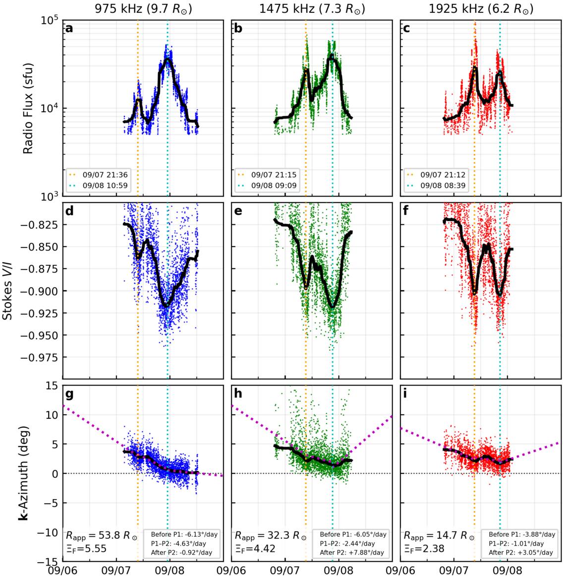
Figure 6. STEREO-A time series at 975 kHz (blue), 1475 kHz (green), and 1925 kHz (red). Top: radio flux with smoothed trend and two broad maxima (P1, P2). Middle: degree of circular polarization V/I (negative values correspond to left-hand polarization in the STEREO/WAVES convention), reaching ∣V/I∣ ≳ 0.9 near the peaks. Bottom: wavevector azimuth with three linear fits (magenta) between P1 and P2, whose slopes yield the apparent rotation radii Rapp and the frequency-dependent scattering factors ΞF quoted in the text.
Download figure:
Standard image High-resolution image2.4. Quasiperiodic Pulsations and Magnetoseismology
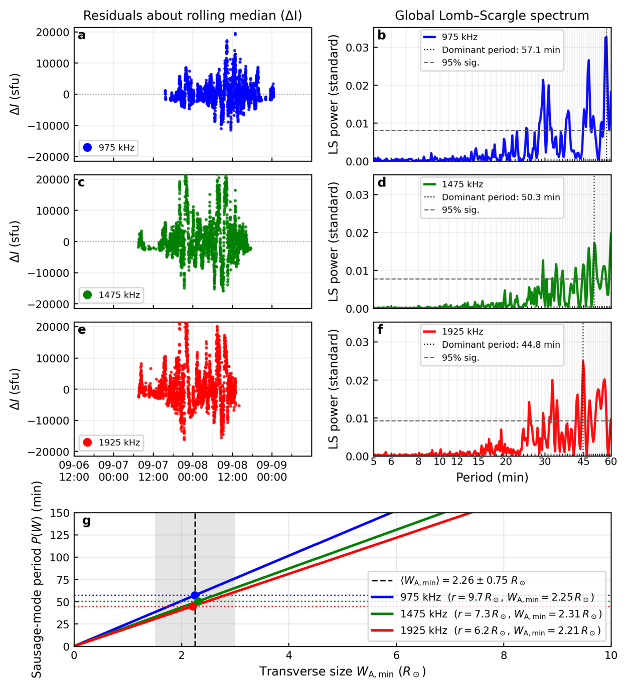
To isolate quasiperiodic pulsations, we remove slow trends from Stokes I by subtracting a 256 minute running median, yielding residuals ΔI(t) (Figures 7(a),(c),(e)). The quasiperiodic pulsation periodograms are computed over the same time intervals shown in Figures 7(a)–(e), selected by the high-confidence thresholds I > 5 × 10³ sfu and V/I < −0.8 (Section 2.3). The P1/P2 times marked in Figure 6 are retained only as visual guides to the broad envelope and are not used as inputs to the periodogram analysis. Lomb–Scargle periodograms (J. D. Scargle 1982) over 5–60 minutes show the highest-power peaks at 57.1 minutes (975 kHz), 50.3 minutes (1475 kHz), and 44.8 minutes (1925 kHz) (Figures 7(b), (d), (f)); the modulation persists for multiple cycles (at least 3–4) over this high-confidence interval. Given potential red noise (i.e., excess low-frequency/background power that can bias periodograms at long periods), we treat these as characteristic and use them to derive a lower bound on the trap size (Equation 4).

Figure 7. Quasiperiodic pulsations and magnetoseismology during the high-confidence portion of Window 3 selected by I > 5 × 10³ sfu and V/I < −0.8 (Section 2.3). (a), (c), (e) Stokes I residuals  after subtracting a 256 minutes running-median trend; the red curve is a smoothed envelope highlighting the oscillations. (b), (d), (f) Lomb–Scargle periodograms of
  computed from the residual time series shown in panels (a), (c), (e) show dominant periods P of 57.1, 50.3, and 44.8 minutes at 975, 1475, and 1925 kHz (vertical dashed lines). Dashed horizontal lines indicate the 95% false-alarm level. Periodograms are evaluated over periods of 5–60 minutes (the plotted range). (g) Panel (g) explicitly shows how the measured period P maps, through the adopted vA(r) model, to the lower bound
  and hence to the minimum half-width
  .
.
Download figure:
Standard image High-resolution imageWe interpret the quasiperiodic pulsations as MHD eigenmodes of a long-lived magnetic trap (H. Rosenberg 1970; V. V. Zaitsev & A. V. Stepanov 1975; V. M. Nakariakov & V. F. Melnikov 2009; I. V. Zimovets et al. 2021). For a cylindrical trap supporting the fundamental fast sausage mode (azimuthal number m = 0), the longest allowed period occurs near the long-wavelength cutoff of the sausage dispersion relation and equals
with j0,1 ≈ 2.4048 the first zero of J0 (P. M. Edwin & B. Roberts 1983; B. Roberts et al. 1984; V. M. Nakariakov et al. 2003; M. J. Aschwanden et al. 2004). Inverting Equation (3) for a measured P yields a conservative lower bound on the transverse size of a sausage-mode trap,
We evaluate vA(r) at the band-specific heights using the E. C. Sittler & M. Guhathakurta (1999) density model and a radial field of B(r) ∝ r−2 normalized to 6 nT at 1 au. The in situ np and ∣B∣ at 1 au in Figures 3((f)–(h)) provide heliospheric context but are not a direct validation of the coronal vA(r) used here, which depends on the adopted coronal density model and field scaling.
Using Equation (4) with the measured periods (57.1, 50.3, and 44.8 minutes at 975, 1475, and 1925 kHz), we obtain  ,
,  , and
, and  , and an ensemble mean
  (1σ; uncertainty dominated by field/density systematics). These lower bounds are in good agreement with the rotation-geometry diameter Wrot = (2.50 ± 0.75) R⊙ (Section 2.3), supporting a trap of streamer-top/flux-rope scale (Figure 7(g)).
We note that global trapped sausage modes require loops that are sufficiently short and dense to exceed the long-wavelength cutoff; in long, slender streamer-top structures, the fundamental can be leaky or suppressed, in which case Equation (4) remains a useful lower bound, and the observed oscillation may instead correspond to a higher harmonic or a localized portion of the structure rather than the global fundamental (V. M. Nakariakov et al. 2003; M. J. Aschwanden et al. 2004). The persistence of these oscillations over several cycles suggests they may be continuously driven or reinforced—for example, by energetic particles bouncing within the trap in resonance with the MHD mode (I. V. Zimovets et al. 2021).
2.5. WCRS Localization
Localizing low-frequency sources from one vantage point is challenging because refraction and scattering bend ray paths and because direction-finding solutions are strongly affected by angular broadening. We therefore introduce the WCRS method, which combines (i) the empirically determined scattering factors ΞF(f) from the azimuth sweep (Section 2.3), (ii) an assumed coronal density model to map frequency to radius, and (iii) simple ray-sphere geometry. For readability, we move the full WCRS derivation (coordinate transforms and the ray-sphere solution) to Appendix B; here, we summarize the procedure and the resulting source locations.
Briefly, we correct the STEREO/WAVES direction-finding angles by shrinking their deviation from the Sun–spacecraft line according to ΞF(f), and intersect the resulting back-traced line of sight with the density model shell Rmodel(f) (Appendix B). This wavevector correction is intended to undo the dominant displacement of the apparent arrival direction caused by wave propagation (scattering/refraction) and thereby recover a physically interpretable trajectory. The resulting close-side solutions for 975, 1475, and 1925 kHz are shown in Figures 2(b)–(d).
We do not show the farside intersection branch: in this event, it would place the source in the sector of CME1, which erupted about 2 weeks before the STEREO-A type IV window; solar rotation would carry such a structure far from the observed longitudes, making that association implausible. We therefore interpret the close-side solution as the physically plausible branch for this event.
The point-to-point trajectories at different frequencies are not strictly continuous in time because each location is derived independently from single-spacecraft direction finding at discrete frequencies and times, and residual propagation effects and density model systematics introduce scatter; nevertheless, the ensemble consistently traces the streamer belt.
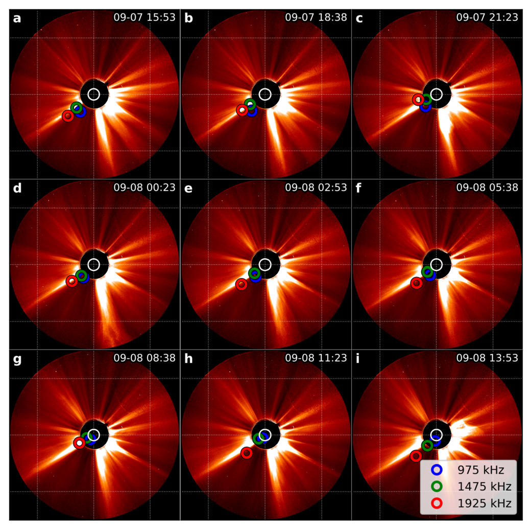
For the white-light context in Figure 8 we show only the wavevector-correction step: we apply the angular shrinking of V. Krupar et al. (2024a) to ϕRTN and θRTN (Equations (B1)–(B2)) and project the resulting corrected arrival directions onto the SECCHI frames. This provides a qualitative check of the association with the helmet streamer; by itself, it does not determine the heliocentric distance (set by Rmodel(f)) or discriminate between the close- and farside intersections along a given line of sight. Small apparent reorderings of the three frequencies in Figure 8 should therefore not be interpreted as true height inversions. They reflect sky-plane projection plus residual propagation scatter within a very broad apparent source (γ ∼ 20°; V. Krupar et al. 2012), so the offset between the plotted centroids is much smaller than the propagation-broadened source extent. The WCRS solutions used for the physical interpretation retain the expected ordering, with the 975 kHz source farther from the Sun than the 1475 and 1925 kHz sources.
Figure 8. White-light context. Coronagraph images spanning the STEREO-A interval with wavevector-corrected direction-finding angles overplotted as angular positions (circles: blue 975 kHz, green 1475 kHz, red 1925 kHz). The corrected directions remain near the helmet streamer apex as the system rotates across the visible hemisphere; these points indicate directions on the sky and are not an independent 3D reconstruction, so their projected distance from the occulter is not a direct proxy for heliocentric source height. An animation of this figure is available. It shows the sequence from 2025 September 6 at 11:53:30 to 2025 September 9 at 11:53:30. The real-time duration is 18 s.
(An animation of this figure is available.)
Download figure:
Video Standard image High-resolution image
We note that (i) the factors ΞF (and ΞH, if harmonics are considered) are taken from the previous subsection for this event; constant fallbacks ΞF ≈ 3.72 and ΞH ≈ 2.10 over 350 kHz–1 MHz are supported by the STEREO survey (V. Krupar et al. 2024a). (ii) All trigonometric functions above take degree arguments; the data products are in degrees throughout. (iii) The WCRS localization used for Figure 2 uses both corrected angles and yields a 3D intersection point on ∣r∣ = Rmodel(f) (Equations (B6)–(B11)); Figure 2 shows the (x, y) projection of the close-side solution, whereas Figure 8 only illustrates the corrected direction of arrival on the plane of the sky.
3.1. A Corotating Electron Reservoir Sustained by CMEs
The observations reveal a hectometric type IV continuum observed over ∼19 days in three successive visibility windows and consistent with corotation with the Sun, becoming visible in sequence to Solar Orbiter, Wind, and STEREO-A as the viewing geometry turns favorable. The strong, nearly pure left-hand circular polarization (∣V/I∣ ≳ 0.9) indicates a single dominant magnetoionic mode in a coherent magnetic environment. This is consistent with coherent emission escaping predominantly in a single magnetoionic mode. Fundamental plasma emission is a natural working assumption (D. J. McLean & N. R. Labrum 1985), but an ECME contribution in an unusually low-density cavity (potentially involving Z-mode waves and mode conversion) also remains plausible (R. M. Winglee & G. A. Dulk 1986a, 1986b; T. Formánek et al. 2025). WCRS localizes the source near the helmet streamer belt at physical heights of order 6–10 R⊙ after propagation is accounted for, a region where large flux ropes and streamer arcades can confine electrons over long intervals. As an order-of-magnitude check, if the emission is plasma radiation at 0.5–3 MHz, the implied densities are ne ∼ 3 × 10³–105 cm−3. Standard Coulomb slowing-down and pitch-angle deflection estimates for ∼20–50 keV electrons then give characteristic collisional times ranging from days at the dense end to months at the tenuous end (J. C. Brown 1972; A. G. Emslie 1978). Coulomb collisions alone therefore do not obviously preclude multiday confinement, although continued replenishment and escape/transport losses may still be important. We do not infer that the reservoir was already fully established at CME1; rather, CME1–CME3 are treated as plausible contributors to sustaining or replenishing the trapped population over the full 19 day interval.
Our WCRS height inference uses a plasma-frequency mapping (fundamental/harmonic); if the emission instead tracked the cyclotron frequency, the absolute heights would shift, but the central observational requirements—corotation, a limited visibility window, and a long-lived reservoir repeatedly replenished by CMEs—remain unchanged. Operationally, the same procedure provides (i) shock height–time profiles from type II bursts suitable for CME nowcasting, and (ii) maps of open field connectivity from type III bursts, both from a single vantage point in near real time.
Two independent size diagnostics are mutually consistent: the rotation-based diameter Wrot (Section 2.3) and the magnetoseismic lower bound  (Section 2.5). We therefore adopt a characteristic trap diameter of W ≈ 2.5–3.0 R⊙ (half-width of a ≈ 1.3–1.5 R⊙), with uncertainties dominated by the density model and B(r) assumptions.
Three fast CMEs originated from the same solar sector during the 19 day span of the event. Their timing relative to the continuum suggests that each CME could contribute to sustaining the reservoir by reorganizing the large-scale magnetic environment and either (i) injecting/reaccelerating electrons within the evolving CME/streamer system, and/or (ii) modulating magnetic connectivity so that the source region at the base of the large corotating loop continues to supply electrons over many days. This interpretation aligns with prior associations of type IV emission with CMEs and shocks (M. Pick & N. Vilmer 2008; R. Miteva et al. 2017; A. Mohan et al. 2024). The pronounced type III storm activity near CME2 (Figures 3(c),(d)) further supports sustained electron release from the same sector. Distinguishing between replenishment of a trapped population and quasi-continuous injection from the low corona will require dedicated modeling and/or energetic electron measurements, and is left for future work.
3.2. Magnetoseismology of a Giant Coronal Trap
The hour-scale quasiperiodic pulsation provides a seismological handle on the intrinsic transverse size of the emitting trap. Adopting the fundamental cylindrical sausage-mode scaling, P = (π/j0,1) W/vA ≈ 1.31 W/vA, the observed periods imply conservative lower bounds on W of only a few solar radii—consistent with the rotation-geometry estimate (Section 2.3) and characteristic of streamer-top/flux-rope structures at r ∼ 6–10 R⊙. Together with the large apparent-to-geometric factor  and the weak frequency dependence of the apparent half-width (Section 3.3), this indicates that propagation (scattering) dominates the measured goniopolarimetric size, while rotation geometry and magnetoseismology recover the intrinsic scale. We note that trapped global sausage modes require sufficiently short, dense loops in long, slender streamer-top configurations. The fundamental may be near cutoff or partially leaky, so the seismological widths should be interpreted as lower bounds, with localized or higher-harmonic oscillations remaining tenable (P. M. Edwin & B. Roberts 1983; B. Roberts et al. 1984; V. M. Nakariakov et al. 2003; M. J. Aschwanden et al. 2004). Alternative MHD interpretations include kink-mode modulation of the emissivity, which can also generate quasiperiodic pulsations in radio light curves (D. Y. Kolotkov et al. 2018).
3.3. Comparison with the 2002 Long-duration Type IV and Disappearing Wind Context
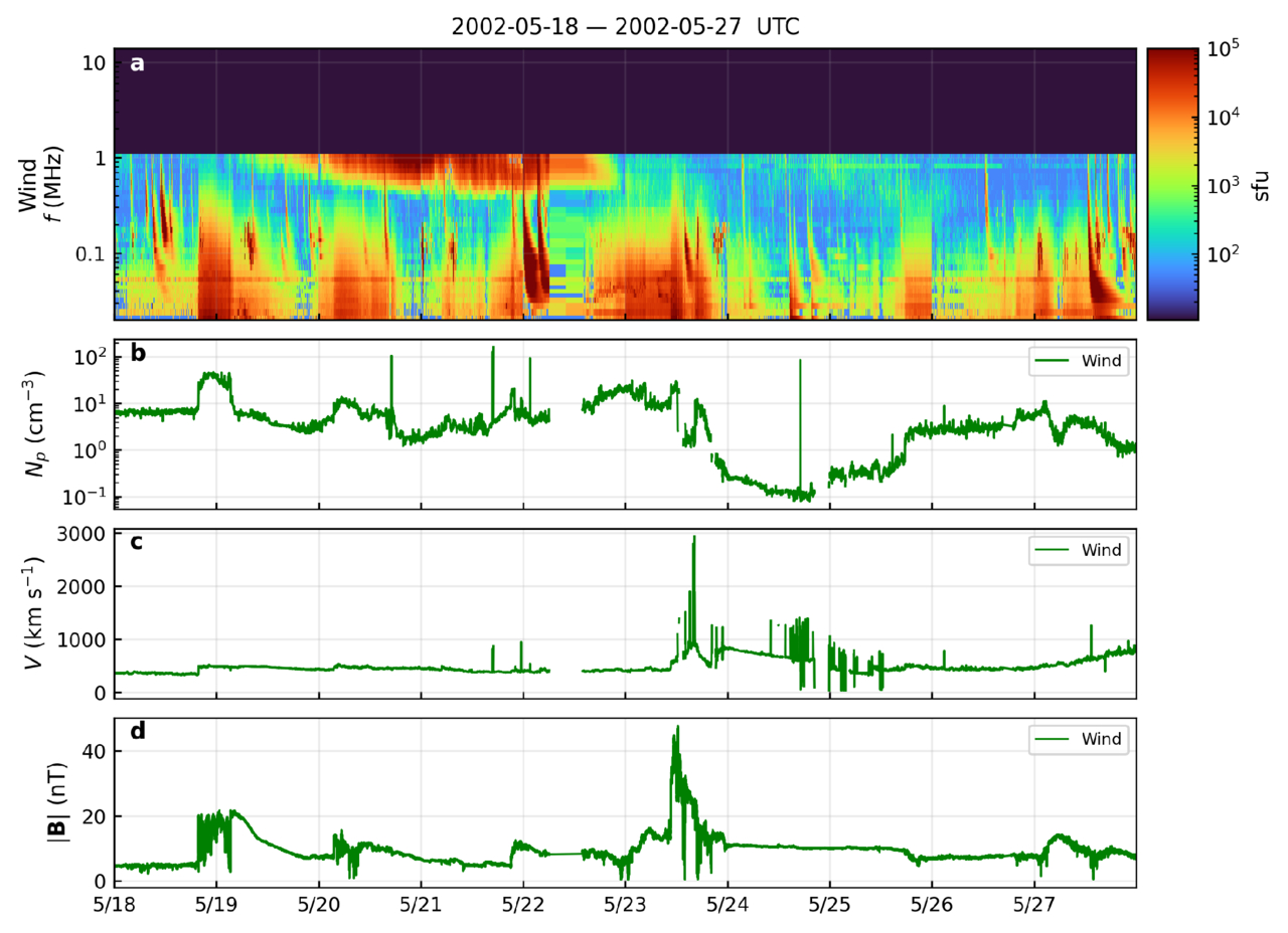
The 19 day corotating continuum reported here echoes the ∼6 days, nearly pure LHC hectometric type IV of 2002 May 17–23 (M. J. Reiner et al. 2006). In both cases, fast/wide CMEs preceded or accompanied the continuum, and the peak phase featured hour-scale quasiperiodic pulsations consistent with standing MHD eigen-oscillations in a large coronal resonant cavity (the electron trap). Importantly, in both epochs the continuum was followed at Earth by an extremely low-density solar wind interval—for 2025 after CME 3 (Figure 3(f)), and for 2002 within ∼1–2 days after the radio maximum ( Appendix C). In the 2002 case, the deepest density dropout occurs after the main ICME signatures (enhanced ∣B∣ and VSW; Figure 9), suggesting a trailing rarefaction/wake rather than the ICME body itself. This repeated ordering suggests that the radio reservoir and the subsequent “disappearing wind” interval may be linked to an over-expanded ICME cavity together with its rarefied wake: the cavity/streamer-top structure can confine and reenergize electrons as it corotates, while the wake reduces scattering/absorption and enhances detectability. The large apparent-to-true size ratio ( ) we measure here further implies that such events are most conspicuous when propagation through the rarefied wake is unusually transparent; under typical, more turbulent conditions, scatter broadening and depolarization may render analogous reservoirs harder to detect from a single vantage point.

Figure 9. 2002 May 18–27: (a) Wind/WAVES dynamic spectrum (sfu) showing the multiday continuum associated with the 2002 May 17–23 type IV reported by M. J. Reiner et al. (2006). (b)–(d) Wind proton density np, bulk speed VSW, and magnetic field strength ∣B∣. Following the ICME on May 23–24 (enhanced ∣B∣ and VSW), Wind encountered an ultralow-density interval with np ≈ 0.1 cm−3 on May 24–25 (“disappearing wind”), lagging the radio maximum by ∼1–2 days.
Download figure:
Standard image High-resolution image3.4. Single-spacecraft Localization Enabled by WCRS
Localizing low-frequency sources from one vantage point is challenging because refraction/scattering bends ray paths. In this event, we used the measured azimuthal drift to determine an event-specific, frequency-dependent scattering factor ΞF(f) and applied angular shrinking to the RTN direction-finding angles before solving the Sun–spacecraft-source geometry on Rmodel(f). The derived values span ΞF ∼ 2.4 (1925 kHz) to ∼5.6 (975 kHz), consistent with stronger scattering at lower fpe. Without this correction, the back-traced ray frequently fails to intersect the density model sphere (no real ray-sphere solution; Equation (B12)), and naive use of the uncorrected angles would bias inferred source heights outward. WCRS thus provides actionable single-spacecraft localizations that complement multispacecraft triangulation and forthcoming imaging, and can be applied in near real time. Operationally, the same procedure may provide (i) shock height–time profiles from type II bursts suitable for CME nowcasting, and (ii) maps of open field connectivity from type III bursts, both from a single vantage point.
3.5. Apparent versus Physical Source Sizes: The Role of 

A key result is the large apparent-to-geometric broadening factor of  measured by STEREO-A, with
  across 1–2 MHz (Section 2.3). We denote the apparent half-width (angular radius) of the source image at the spacecraft by γ (from goniopolarimetric size measurements; V. Krupar et al. 2012), whereas γrot is the geometric half-width inferred from the rotation-based size. The very large
  demonstrates that the apparent extent is dominated by propagation—multipath scattering by solar wind density inhomogeneities—rather than by the intrinsic source size. The near-constancy of γ with frequency, despite changes in modeled source height, further supports a scattering-controlled point-spread function at these frequencies.
The two scattering diagnostics in this work, ΞF(f) from direction-of-arrival deflection and  from broadening, are physically distinct but complementary. ΞF quantifies how far the incoming wavevector is tilted from the true source direction, which must be corrected to recover location and height.
  quantifies how much the apparent image is smeared relative to the true source size. Taken together, the large ΞF at lower frequencies and the event-averaged
  explain why the measured angular sizes (γ ∼ 20°–40°) greatly exceed the physical trap diameter (W ∼ 2.5–3.0 R⊙): the former are propagation-broadened images, whereas the latter reflect the intrinsic geometry constrained by rotation and magnetoseismology.
When an independent geometric width is unavailable (as in many type II/III cases), one may use an empirical  (or the event average of
  ) as a propagation debroadening factor. If γ is the measured goniopolarimetric half-width at the spacecraft, an estimate of the intrinsic transverse diameter is
where DSC is the Sun–spacecraft distance and Rmodel(f) is the modeled heliocentric height of the source at frequency f. Thus,  provides a simple, instrument-agnostic correction from apparent to physical source size for type II/III bursts at hectometric frequencies where scattering conditions are comparable.
3.6. Limitations and Outlook
Our analysis has some limitations. It relies on single-spacecraft direction-finding and an empirical scattering correction. The absolute source heights inherit uncertainties from the coronal density model (and our assumed B(r) ∝ r−2 scaling). We also assumed a constant ΞF(f) over the multiday interval, and any uncorrected polarization calibration offsets could introduce additional systematic error. Nevertheless, multiple independent observations—the multispacecraft visibility sequence, the strong circular polarization in one mode, the agreement between rotation-based and magnetoseismic sizes, and the consistency of WCRS-derived positions with helmet streamer geometry—all converge to the same interpretation: a long-lived coronal electron reservoir.
Methodologically, our WCRS approach enables single-spacecraft radio source localization today, and it will synergize with radio imaging by upcoming missions like SunRISE (J. Lazio et al. 2017). By combining WCRS with imaging data and in situ particle measurements, future studies can more precisely quantify how CMEs seed and maintain such heliospheric electron reservoirs, improving both our physical understanding and space-weather monitoring capabilities.
3.7. Concluding Remarks
The observations and analysis link, to our knowledge, the longest reported hectometric type IV continuum to a corotating electron reservoir, and show how frequency-aware propagation corrections can yield a physically interpretable single-spacecraft localization estimate.
Event-specific observational/physical conclusions:
1.
Record-long hectometric type IV. To our knowledge, we observed the longest reported hectometric type IV continuum, spanning 0.5–3 MHz across three successive visibility windows over nearly 19 days at four spacecraft spread across 220° longitudinally.
2.
Sustained reservoir. Three fast CMEs from the same solar sector plausibly helped maintain the reservoir by restructuring the large-scale trap and enabling continued electron injection from the low corona.
3.
Recurring pattern across cycles. A possible recurring pattern across solar cycles may exist: the 2025 event shares strong polarization, hour-scale quasiperiodic pulsations, and a subsequent rarefied solar wind interval with the 2002 May 17–23 event (M. J. Reiner et al. 2006). This suggests (but does not prove) that over-expanded CME/ICME cavities and their rarefied wakes could both confine/reenergize electrons and reduce propagation blurring, enhancing hectometric type IV visibility; testing this hypothesis will require a larger event sample.
Methodological contribution (WCRS) and scope/implications:
1.
Single-spacecraft localization. Using a frequency-dependent scattering correction (WCRS), a single spacecraft can provide an event-specific localization estimate for low-frequency sources. In this event, WCRS places the source near a helmet streamer at a physical height of ∼6–10 R⊙.
2.
Intrinsic size from two diagnostics. Solar rotation geometry and sausage-mode magnetoseismology (P = (π/j0,1)W/vA) are consistent with an intrinsic transverse width of only a few solar radii, W ≈ 2.5–3.0 R⊙ (with the seismology providing a lower bound).
3.
Propagation-dominated image. The apparent goniopolarimetric half-width is much larger than the inferred intrinsic width (B ∼ 60 ± 18), showing that interplanetary scattering strongly affects the observed source extent in the 1–2 MHz band.
4.
Outlook. WCRS and MHD seismology provide powerful single-spacecraft diagnostics. Coupling these with forthcoming low-frequency imaging (e.g., SunRISE) and in situ particle data will sharpen constraints on source geometry and energetics, including shock height–time profiles from type II lanes and connectivity maps from type III ensembles, enhancing our space-weather forecasting toolkit.
Solar Orbiter is a mission with international cooperation between ESA and NASA, operated by ESA. The RPW instrument was designed and funded by CNES, CNRS, the Paris Observatory, the Swedish National Space Agency, ESA-PRODEX, and all participating institutes. Parker Solar Probe was designed, built, and is now operated by the Johns Hopkins Applied Physics Laboratory as part of NASA’s Living With a Star (LWS) program (contract NNN06AA01C). We gratefully acknowledge the STEREO/WAVES and Wind/WAVES instrument teams and the mission operations teams for maintaining high-quality, openly available data products. V.K., O.K., and L.K.J. are supported by the STEREO mission. H.R. acknowledges UKSA grant Nos. ST/X002012/1, UKRI980, and STFC grant No. ST/W001004/1. All spacecraft data used in this study are publicly available from NASA’s Space Physics Data Facility (SPDF) at https://spdf.gsfc.nasa.gov/. This work utilizes data produced collaboratively between the Air Force Research Laboratory (AFRL) and the National Solar Observatory (NSO). The ADAPT model development is supported by AFRL. The input data utilized by ADAPT is obtained by NSO/NISP (NSO Integrated Synoptic Program). NSO is operated by the Association of Universities for Research in Astronomy (AURA), Inc., under a cooperative agreement with the National Science Foundation (NSF). The authors acknowledge K. Issautier, French PI of the Wind/WAVES instrument and the French CDPP database for the Wind/RAD1 and RAD2 L2 data distribution. This research has made use of the Astrophysics Data System, funded by NASA under Cooperative Agreement 80NSSC25M7105. The authors thank Therese A. Kucera (NASA/GSFC) for insightful discussions related to the analysis of STEREO data and the resulting interpretation.
We convert the Level-2 voltage power-spectral density PV(f) (V2 Hz−1) to the incident spectral flux density S(f) (W m−2 Hz−1) with the short-dipole relation

where Z0 ≃ 377 Ω is the impedance of free space and ΓLeff(f) (m) is the reduced effective length that maps the open-circuit antenna voltage to the ambient electric field in the short-dipole limit (L ≪ λ), assuming unpolarized emission and a wavevector nearly orthogonal to the dipole axis (A. Zaslavsky et al. 2011). The same conversion in Equation (A1) is applied to Solar Orbiter/RPW and to Wind/WAVES. We report fluxes in solar flux units (sfu),
i.e., all spectra are normalized to 1 au by inverse-square scaling. We adopt STEREO-A/WAVES as the absolute flux etalon (J. L. Bougeret et al. 2008; V. Krupar et al. 2022); during short separation intervals, we solve Equation (A1) for ΓLeff(f) by matching type III burst fluxes to STEREO-A after the 1/r2 renormalization. The 1/r2 falloff has been verified for radially aligned spacecraft over ∼ 50 R⊙ to 1 au (V. Krupar et al. 2024b). We also calculate the receiver background as the lowest 1% value per channel over 1 day and subtract it frequency by frequency from Ssfu(f); this produces the background-subtracted spectra shown in Figures 1 and 3.
A.1. Solar Orbiter/RPW
RPW acquires electric spectra with the TNR (∼4 kHz–1 MHz) and the HFR (0.375–16 MHz) operating in dipole mode using the V1, V2, and V3 booms (M. Maksimovic et al. 2020). Narrowband spacecraft disturbances—most prominently at ∼80 kHz (reaction wheels) and ∼120 kHz (PCDU) with harmonics—contaminate parts of the band; therefore, all flux conversions are restricted to the vetted clean channel lists compiled for Solar Orbiter operations (M. Maksimovic et al. 2021).
Our calibration strategy deliberately builds on and extends the approach of A. Vecchio et al. (2021): that study established an in-flight cross-calibration from only three relatively weak type III bursts, using Wind/WAVES RAD1 flux as the reference and deriving reduced effective lengths ΓLeff. Here, we adopt STEREO-A/WAVES (J. L. Bougeret et al. 2008; V. Krupar et al. 2022) as the absolute flux etalon and enlarge the calibration set to 12 near-alignment type III intervals between 2022 November 22 and 2022 December 3. For each clean frequency, we solve the short-dipole inversion frequency by frequency so that the 1 au renormalized RPW flux matches STEREO-A. Combining all events yields more stable, higher-fidelity ΓLeff(f) estimates across the TNR/HFR bands (including the mild high-frequency roll-off), with uncertainties taken as the event-to-event scatter. The adopted ΓLeff(f) values used throughout this Letter are summarized in Table 1.
Table 1. Solar Orbiter/RPW Dipole Gains Used in This Work: ΓLeff (m)
| RPW Dipole | ΓLeff for f ≤ 2000 kHz | ΓLeff for f > 2000 kHz |
|---|---|---|
| V1–V2 | 2.903 ± 0.184 |
![$(2.903\pm 0.184)\,\exp \,\left[1.514\times 1{0}^{-4}(f-2000)\right]$](https://content.cld.iop.org/journals/2041-8205/1003/1/L5/revision1/apjlae5537ieqn50.gif)
|
| V2–V3 | 2.410 ± 0.186 |
![$(2.410\pm 0.186)\,\exp \,\left[1.369\times 1{0}^{-4}(f-2000)\right]$](https://content.cld.iop.org/journals/2041-8205/1003/1/L5/revision1/apjlae5537ieqn51.gif)
|
| V3–V1 | 2.925 ± 0.175 |
![$(2.925\pm 0.175)\,\exp \,\left[1.472\times 1{0}^{-4}(f-2000)\right]$](https://content.cld.iop.org/journals/2041-8205/1003/1/L5/revision1/apjlae5537ieqn52.gif)
|
Note. The left column applies below 2 MHz; the right column gives the frequency dependence above 2 MHz (f in kHz).
Download table as: ASCIITypeset image
Table 2. Wind/WAVES Reduced Effective Lengths ΓLeff (m) from STEREO-A Cross-calibration of 19 Type III Bursts (2023 August)
| Channel | RAD1: 20–1040 kHz | RAD2: f ≤ 2500 kHz | RAD2: f > 2500 kHz (with f in kHz) |
|---|---|---|---|
| S | 30.510 ± 1.526 | 6.272 ± 0.314 |
![$(6.272\pm 0.314)\,\exp \,\left[8.15\times 1{0}^{-5}\,(f-2500)\right]$](https://content.cld.iop.org/journals/2041-8205/1003/1/L5/revision1/apjlae5537ieqn53.gif)
|
| SP | 30.620 ± 1.531 | 6.529 ± 0.326 |
![$(6.529\pm 0.326)\,\exp \,\left[4.905\times 1{0}^{-5}\,(f-2500)\right]$](https://content.cld.iop.org/journals/2041-8205/1003/1/L5/revision1/apjlae5537ieqn54.gif)
|
| Z | 3.163 ± 0.158 | 2.706 ± 0.135 |
![$(2.706\pm 0.135)\,\exp \,\left[6.95\times 1{0}^{-5}\,(f-2500)\right]$](https://content.cld.iop.org/journals/2041-8205/1003/1/L5/revision1/apjlae5537ieqn55.gif)
|
Download table as: ASCIITypeset image
A.2. Wind/WAVES
Wind/WAVES acquires radio autospectra with two swept receivers (J.-L. Bougeret et al. 1995), RAD1 (20–1040 kHz) and RAD2 (1.075–13 MHz), using three orthogonal electric sensors (X, Y, Z). A front-end switching/matrix selects S, SP, and Z channels with different antenna couplings in the two bands: in RAD1, the S/SP chains sample the spin-plane path (SEP mode; ≈X), whereas in RAD2, the S/SP chains sample a summed path (SUM mode; ≈X + Z). SP is the 90° quadrature replica of S for goniopolarimetry; Z is the spin-axis monopole in both bands (J.-L. Bougeret et al. 1995). These mode differences (SEP versus SUM) and their distinct impedance/matching paths lead to different reduced effective lengths ΓLeff for RAD1 and RAD2, even for the same labeled channel.
As for Solar Orbiter, we use STEREO-A/WAVES as the absolute flux etalon. We selected 19 type III bursts occurring during 2023 August 2 to 2023 August 20 with longitudinal separations of <1°. For each event, we distance normalize both instruments by (1 au/r)2, and determine ΓLeff(f) so that the WAVES flux reproduced via Equations (A1) and (A2) matches the STEREO-A flux at the nearest channel. We use Z for the science analysis in Figures 1 and 3 (least affected by spin/mode artifacts); S/SP are reported here for completeness (Table 2).
To localize the source in 3D heliocentric coordinates, we intersect a wavevector-corrected line of sight from the spacecraft with a density model sphere (WCRS). The observed radio frequency constrains the local plasma frequency and hence the radial height via a coronal density model; we adopt the method in E. C. Sittler & M. Guhathakurta (1999) for Rmodel(f). Interplanetary refraction/scattering tilts the measured wavevector away from the nearly radial source direction, so the raw angles from direction finding cannot be used directly. We therefore apply angular shrinking with the relative deviation factor ΞF(f) obtained in the previous subsection (fundamental emission; harmonic uses ΞH). For reference, a statistical survey of interplanetary bursts found nearly frequency-independent median values ΞF ≈ 3.72 (fundamental) and ΞH ≈ 2.10 over 0.35–1 MHz (V. Krupar et al. 2024a). Thus, our use of an event-specific, frequency-dependent ΞF(f) follows the empirical remedy advocated in those studies for correcting single-spacecraft direction-finding data.
We work with the RTN azimuth ϕRTN and colatitude θRTN (both in degrees) and shrink the angular deviations multiplicatively:
We avoid the term offset, since the correction is a shrink (divide) of a deviation, not an additive shift.
The direction-finding product provides (ϕRTN, θRTN) in the spacecraft RTN basis. To express the corresponding corrected wavevector in a heliocentric Cartesian basis, we (i) construct the RTN triad in that basis from the spacecraft ephemeris and a north reference axis, and then (ii) expand the spherical angles on that triad. We implement the calculation in HEEQ, but the same algebra applies in other Sun-centered Cartesian frames (e.g., HEE, and in principle, HCI), provided the spacecraft position rSC(t) and the reference axis used to define the RTN  direction (here, the solar rotation axis) are expressed consistently in that frame.
Let the spacecraft heliocentric position in HEEQ Cartesian coordinates be rSC(t) = (xSC, ySC, zSC), with DSC = ∣rSC∣. We form an RTN triad expressed in the same HEEQ basis via


where  is the fixed HEEQ north unit vector (solar rotation axis). In this convention, ϕRTN is measured in the
  –
– plane from
  toward
  , and θRTN is colatitude measured from
  (0° at
  , 90° in the
  –
– plane).
The corrected unit wavevector (direction of propagation from the source to the spacecraft) expressed in HEEQ is
and the back-traced ray direction from the spacecraft toward the source is

We then intersect the ray  with the density model sphere ∣r∣ = Rmodel(f). Solving
  yields the quadratic

with  ,
,  , and
, and  . The solutions are
corresponding to the near (“close-side”) and far (“farside”) solutions along the same line of sight. The corresponding heliocentric source positions are


In this work, we use the close-side solution for the quantitative localization and in Figure 2; the farside solution is retained for completeness but is not otherwise interpreted here.
A real intersection exists only when the discriminant in Equation (B9) is nonnegative, i.e., B2 − AC ≥ 0. For unit vectors, this condition is equivalently
where ψcorr is the corrected angular separation between the incoming ray and the Sun–spacecraft line. At ∼1 au, DSC/Rmodel(f) ≫ 1, while ψ is typically several degrees, so Equation (B12) is often violated without shrinking. Dividing by ΞF restores a real-valued intersection; this is the same empirical remedy advocated for interplanetary bursts in the 0.35–1 MHz band (V. Krupar et al. 2024a).
Equations (B1)–(B11) are the operations used to build the colored trajectories in Figures 2(b)–(d): we compute rsrc,close(t, f) on the sphere ∣r∣ = Rmodel(f) and plot its projection onto the HEEQ equatorial (x–y) plane.
Figure 9 shows the Wind/WAVES dynamic spectrum with in situ plasma and magnetic field measurements to illustrate the temporal offset between the multiday type IV continuum in 2002 and the ultralow-density solar wind interval that followed at 1 au. As reported by M. J. Reiner et al. (2006), the 2002 event persisted for nearly 6 days, was essentially purely left-hand circularly polarized, and spanned at least 0.4–7 MHz with hour-scale quasiperiodic pulsations and drifting narrowband structure. In Figure 9(a) (quicklook), we can identify the extended continuum and its decline by approximately May 22–23.
The in situ context at Wind (Figures 9(b)–(d)) shows the expected ICME passage on May 23–24 (enhanced ∣B∣ and VSW), followed within the next ∼1 day by a pronounced rarefaction: the proton density dropped to np ≈ 0.1 cm−3 for ≳ 12–24 hr (May 24–25), i.e., a transient “disappearing solar wind” interval. Thus, as in our 2025 case, the chronology is type IV → ICME → rarefied wake: a long-lived, corotating radio continuum precedes an ultralow-density interval at Earth by ∼1–2 days. The fact that the density minimum lags the ICME interval suggests that the rarefaction resides in the trailing wake rather than within the ICME body itself. Together with the 2025 observations, this historical example supports the interpretation that over-expanded ICMEs can create a coupled cavity-wake system in which (i) the ICME/streamer-top magnetic structure provides a large, long-lived electron trap that sustains the type IV reservoir, while (ii) the trailing rarefied wake reduces propagation blurring along the line of sight, making continua unusually conspicuous when it intersects the observer’s view.