Since the first experimental realisation of Bose–Einstein condensation in dilute atomic gases [1–3]—one of the most precisely controllable quantum many-body systems—these systems have become important platforms for quantum simulation [4–6], precision metrology [7–9], and emerging quantum technologies [10, 11]. Central to these applications is the precise thermodynamical characterisation—particularly values of the temperature and chemical potential—which, in thermal equilibrium under the grand canonical ensemble, fully determine the system’s quantum statistical state and collective behaviour.
Conventionally, the temperature and chemical potential in ultracold atomic experiments are extracted using destructive time-of-flight imaging techniques [12–14]. In this method, the trapping potential is abruptly switched off, allowing the atomic cloud to expand freely. The temperature is then inferred from the spatial distribution of the cloud, assuming a Maxwell–Boltzmann velocity distribution. For a cloud with a Gaussian density profile, the  width in the trap, σ0, and the
  width after a time of flight t, σ, are related by
  , where m is the atomic mass. However, this approach is inherently destructive and suffers from significant shot-to-shot variability, limiting experimental reproducibility and precision. Furthermore, the Maxwell–Boltzmann approximation is fundamentally unsuitable for describing quantum degenerate gases, which exhibit significant quantum statistical correlations and non-trivial interactions.
Minimally invasive thermometry approaches that use impurity-based polarons have been proposed and shown to be capable of nanokelvin and subnanokelvin precision by analysing impurity fluctuations in momentum and position [15–17].
In this paper, we demonstrate a proof-of-principle, minimally destructive thermometric technique using machine learning. Our method directly estimates temperature and chemical potential from in situ density profiles, facilitating repeated, rapid measurements on the same atomic sample without significantly perturbing it. Our approach is inspired by recent advances in machine learning to classify and characterise quantum fluid states [18–21]. Fundamentally, we learn the highly non-trivial mapping from a condensate’s atomic density to the thermodynamical parameters of interest—this is beyond what is possible in naïve fitting procedures currently used in cold atom experiments. We train our machine learning model using simulated density distributions generated from the stochastic Gross–Pitaevskii equation (SGPE), a theoretical framework for modelling finite-temperature dynamics and thermal fluctuations in Bose gases.
We validate our approach across a broad range of temperatures and chemical potentials, and evaluate its estimating capability using unseen density profiles with varied trapping geometries (despite only being trained on harmonically trapped condensates) and during thermalisation (despite only being trained on thermally equilibrated density profiles). Our results demonstrate the robustness and versatility of machine learning thermometry, suggesting its potential as a powerful, precise, and experimentally feasible tool for the investigation of ultracold atomic systems.
2.1. Dynamical treatment of the condensate
The theoretical treatment of a dilute Bose gas begins with the many-body Hamiltonian

where

incorporates the single-particle kinetic energy and the external trapping potential  , and
, and  represents the two-body interatomic potential, where the factor 1/2 prevents double-counting of particle interactions.
Despite the strong short-range interactions characteristic of alkali atoms, ultracold gases of these species can be treated as weakly interacting systems [22]. At very low temperatures, the de Broglie wavelength λ greatly exceeds the range of the interatomic potential, permitting the approximation of interactions as elastic, point-like contacts characterised by the s-wave scattering length. This leads to the pseudopotential approximation  , where the interaction strength
  is directly proportional to the scattering length as.
The Heisenberg equation of motion for the Bose field operator  is given by

We decompose the field operator into condensate and non-condensate contributions [23]:

where  describes the condensate atoms and
  represents non-condensate atoms (thermal excitations, quantum fluctuations, or both); unlike the field operator
  , condensate dynamics mean these may both have an explicit time-dependence. In the limit of large condensate occupation, the ensemble average reduces to a classical field:
  , such that
  .
.
Substituting this decomposition into (3) and taking the expectation value yields a form of nonlinear Schrödinger equation

In the limit of negligible fluctuations, this reduces to the Gross–Pitaevskii equation, which provides an accurate description for weakly interacting gases with large atom numbers at temperatures typically below half the critical temperature for Bose–Einstein condensation.
2.2. Dynamics of Bose gases at finite temperatures
To investigate Bose gas dynamics across a broader temperature range, including near the phase transition, we require a treatment that incorporates thermal fluctuations beyond the mean-field approximation of (5).
We choose to model the growth of the condensate with the SGPE [24–27], which describes a static coupling of the condensate modes to a thermal bath. The growth is towards a state that corresponds to a thermodynamical equilibrium in the grand canonical ensemble defined by our choice of µ and T, which, by definition, must take real values. In essence, the SGPE is a phenomenologically damped Gross–Pitaevskii equation with additive noise. This approach implements a fluctuation–dissipation theorem that ensures the system relaxes to the correct equilibrium state, without spurious enhancement or depletion of either condensate or thermal components. The SGPE takes the form

where

is commonly referred to as the Gross–Pitaevskii ‘Hamiltonian,’ and the Gaussian noise correlations satisfy

note  is a classical noise term, hence the angle brackets in (8) describe a purely statistical averaging, and not an expectation value over a quantum state.
We use a fourth-order Runge–Kutta scheme to solve equation (6) on a discretised spatio-temporal grid. There is an implicit projection out of high-momentum modes which are beyond the maximum momentum the spatial grid may represent. Under the numerical scheme as described in equations (6)–(8), we do not consider any interactions with the thermal cloud, i.e. we neglect an additive term  in equation (7) for the incoherent mean-field contribution (where
  is the non-condensate density and the factor of 2 arises from exchange symmetry under a Hartree–Fock theory). Such a term is important for quantitative agreement with experiments; for further discussion see e.g. [28, 29].
Since our focus lies in generating equilibrium thermal states rather than studying formation dynamics, the precise value of the dimensionless coupling parameter γ is not critical. This parameter controls how quickly the system equilibrates with its thermal environment—smaller values lead to slower equilibration, while larger values speed it up proportionally. However, γ must be chosen carefully: too small and the simulation becomes computationally impractical; too large and topological defects can form, actually slowing convergence. We use a spatially uniform rate γ = 0.01 throughout our simulations, which provides a good balance between computational efficiency and physical accuracy.
We evolve the system until we reach thermal equilibrium, as monitored by the relative change in condensate number:

We assume equilibrium to have been achieved when  for five consecutive time steps.
For machine learning purposes, we partition the resulting atomic density profiles into three datasets: 80% for training, 10% for validation during each epoch, and 10% for final testing. The model is never exposed to the validation or test datasets during training. We use the training set to optimise the model parameters, the validation set to monitor generalisation and prevent overfitting during training, and the test set to provide an unbiased estimate of final performance on unseen data.
2.3. Atomic species and trap geometry
We consider ultracold, single-species atomic Bose gases of rubidium 87 with scattering length  [30] and atomic mass
  . The temperatures are sampled from
  , encompassing both deeply degenerate and near-critical regimes. Chemical potentials are sampled from
  rather than from a regular grid to ensure robust model generalisation. Additional parameters are documented in our open-source code [31].
We use highly anisotropic trapping geometries. For harmonic traps, the potential is  with transverse frequencies
  and axial frequency
  . We introduce a slight random anisotropy3 in the transverse dimensions to emulate experimental imperfections. We also consider toroidal traps with potential
 ![$V(x,y,z) = V_0 \{1-\exp( -\sigma^{-2}[\rho(x,y,z)-R]^2 ) \}$](https://content.cld.iop.org/journals/2632-2153/7/2/025047/revision2/mlstae4f4fieqn27.gif) , where V0 is the trap depth, ρ is the radial distance from the torus centre, and σ and R are the minor and major radii, respectively.
, where V0 is the trap depth, ρ is the radial distance from the torus centre, and σ and R are the minor and major radii, respectively.
In our model training we use quasi-two-dimensional (2D) condensates with an assumed Gaussian profile in the strongly confined z-dimension, except in section 4.2, where we test the model on column-integrated three-dimensional (but still highly anisotropic) condensates. The assumed tight axial confinement is equivalent to requiring  and
and  . The z-dimensional contribution is the harmonic oscillator ground state
  , yielding the complete field
  . We can then evolve
  with a 2D equivalent to (6), where g and µ are replaced by the effective 2D parameters
  and
and  .
.
3.1. Overview
We train our model on a set of M = 3000 atomic density profiles,  [where
  ], at thermal equilibrium, each of which is a square image of N rows of N pixels, where N = 256. The network architecture consists of an image processing and feature extraction pipeline followed by a prediction pipeline, as shown in figure 1. This architecture effectively processes the rich spatial information in atomic density profiles—extracting features at various orders of magnitude of the atomic density—to determine a pair of scalar values which we associate with the chemical potential and temperature.
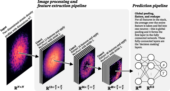
Figure 1. Architecture of the convolutional neural network designed to take the density profile of an atomic Bose–Einstein condensate as an input, and from it determine the condensate’s chemical potential, µ, and temperature, T. The network processes 2D density profiles through three convolutional layers (extracting 12, 24, and 48 features, respectively), each followed by a maximum pooling layer with stride 2 (see appendix
Download figure:
Standard image High-resolution image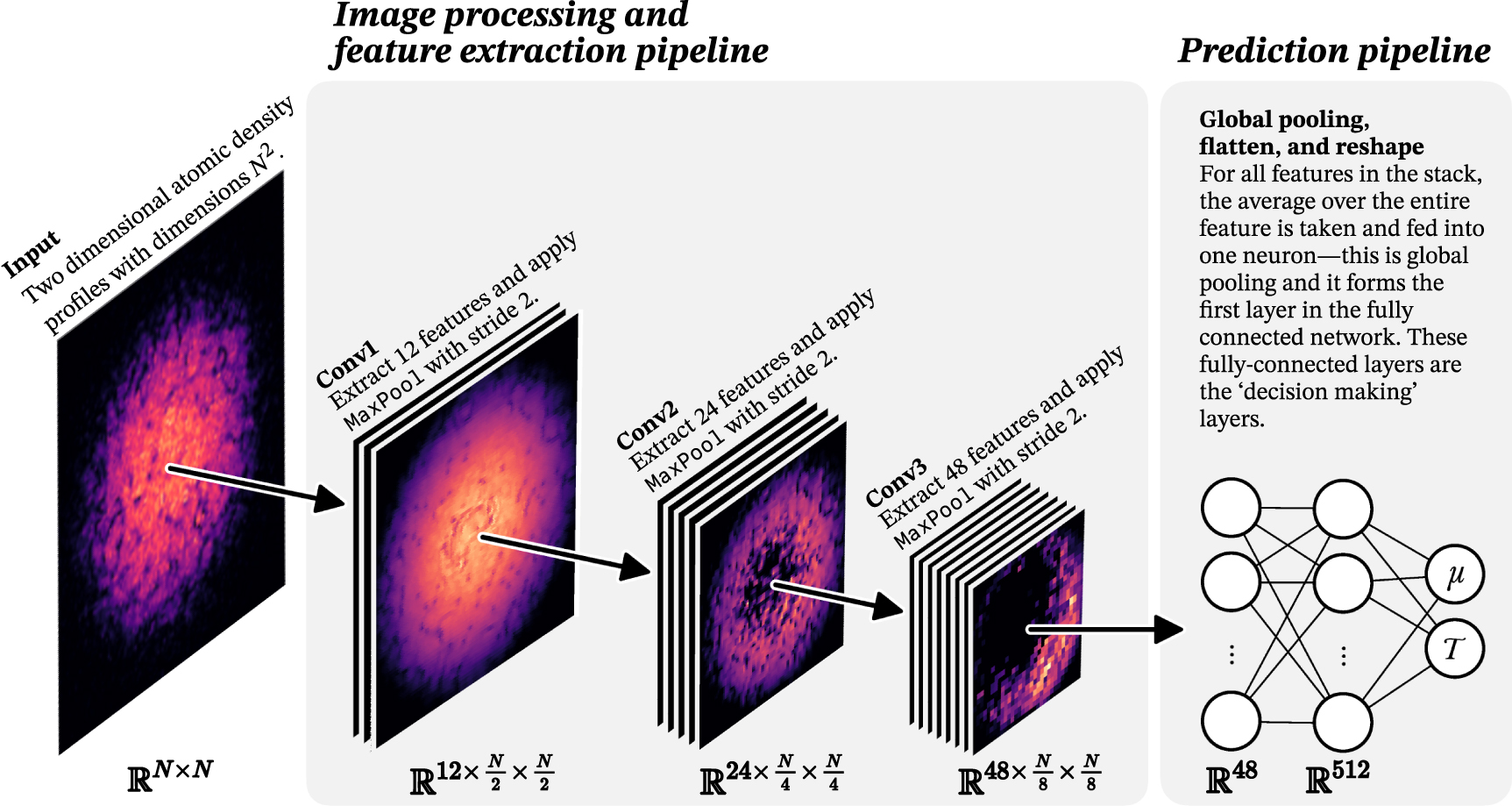
The image processing and feature extraction pipeline consists of three convolutional layers that increase the number of features (layer 1: 12, layer 2: 24, layer 3: 48) to be extracted in each layer, enabling the model to learn from different aspects of the input data (such as different orders of magnitude of the atomic density or any shape or curvature in the condensate). The reduction of spatial dimensions is not only for computational convenience4—by reducing the dimensionality of the input, we force the network to learn local, spatially coherent features and reduce the risk of overfitting (by using fewer parameters—referred to as weights and biases—in the network) [32].
The prediction pipeline transforms the spatial features extracted by the convolutional layers into scalar-valued estimations or ‘predictions’ of the chemical potential and temperature. By averaging each feature map in Layer 4, we reduce the matrix dimensions and capture global information from each feature. We then expand the model’s representational capacity from 48 to 512 neurons in the first fully connected layer (Layer 5 of the overall network)—this layer facilitates complex, highly non-linear combinations of the pooled features, which is essential for mapping the subtle details of the density profiles to the desired thermodynamic parameters. A large number of neurons in this layer improves the model’s predictive and generalisation capabilities—having fewer neurons in this layer was not as conducive to learning (and sufficiently few meant that the network could not determine the values of µ and T within any acceptable error) and more neurons did not appreciably improve our model’s predictive capabilities. There was no further processing in the output layer (e.g. an activation function); an in-principle consequence is the possibility of predicted negative values for the chemical potential (which can be meaningful, although not in the systems we consider) and the temperature (which is not meaningful). We never observed this to happen, and note that the validity of the SGPE model effectively assumes a finite temperature which is in some sense appreciable.
3.2. Scaled form of the stochastic SGPE
When generating the training data for the model, we consider a scaled system of units in order to avoid computing very small terms (e.g. of the order of  expressed in SI units). In particular, we introduce the following scaling factors: lengths are scaled by the harmonic oscillator lengths
  , times by
  , energies by
  , and temperatures by
  . The condensate field is rescaled as
  , and the position and time variables become
  and
and  respectively, where
  . The Laplacian transforms as
  , while the effective 2D chemical potential and interaction strength are rescaled as
  and
and  . Neglecting the tildes for convenience, the resulting form of the SGPE is:

with equivalently scaled Gaussian noise ensemble correlations

It is these forms that we use to generate all atomic density samples in this work.
In our simulations, we consider a dimensionless spatial step size  , which for the 87Rb system and the
  grid we consider, corresponds to a total grid length of 80 µm. We evolve the system by a maximum of 100 000 time steps (although this is typically much smaller depending upon the dynamical time to thermalisation) using a dimensionless time step size
  . Other simulation parameters (in scaled and unscaled forms) can be found in our source code.
In the following sections, we will first describe the prediction pipeline, starting at layer 4 of the overall neural network, followed by a detailed explanation of the image processing and feature extraction pipeline. We outline the specific mathematical operations used in our convolutional network and contextualise what is often thought of as a ‘black box,’ in a presentation intended to be relevant and accessible for anyone with a physics background.
3.3. Prediction pipeline
The prediction pipeline is a fully connected, feedforward neural network, consisting of three layers, as shown in figure 2. This is preceded by the feature extraction pipeline, which reduces the dimensionality of the input images, through a sequence of three convolutional layers. The output of the feature extraction pipeline consists of 48 features  , which are
  square matrices, i.e.
 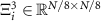 , where
  . Taking the average values over the rows and columns of the 48 features
  produces 48 reduced feature representations
  . These are the input values for the first layer of the prediction pipeline, and the fourth layer overall.
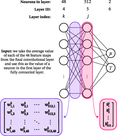
Figure 2. The prediction pipeline architecture, showing in more detail the final part of the network architecture depicted in figure 1. Three fully connected, feedforward layers convert the spatial information from the feature extraction pipeline to a pair of scalar values associated with the chemical potential and temperature, highlighting the weights  between layers and the biases
  associated with the neurons in a layer, for
  .
.
Download figure:
Standard image High-resolution image
In Layer 5, there are 512 neurons with ReLU activation (a necessarily nonlinear function that is commonly used in image recognition scenarios [33]). The pre-activation values are determined from the  through

where we define  as the weight connecting the kth neuron in layer
  to the jth neuron in layer
  , and
, and  as the bias for the jth neuron in layer
  (we use the same notation detailed in appendix A of [34]). We then apply the activation function to produce

These values feed into Layer 6 (the final layer), through

which gives estimations for the chemical potential  and temperature
  , in nanokelvin. We initialise the weights and biases using the Kaiming scheme [35], as
  and
and  (see appendix C in [34] for details). The final layer does not use an activation function, which is motivated by the physics. The chemical potential can be any real value, and the temperature can be any positive, real value, so no activation function is required (one might, in principle, use the
  activation for the temperature, but we did not observe negative temperatures being output from our model)5.
3.4. Image processing and feature extraction pipeline
The input atomic density can be thought of as a monochromatic image described by a matrix  . We show an example in figure 3(a)—while we display it using a false colour scale, in terms of information (each pixel has a single value assigned to it, describing the local density) it is functionally monochromatic. The image is processed through three convolutional layers, each followed by ReLU activation and maximum pooling (MaxPool). Figure 3 demonstrates intermediate steps to calculate a single feature from the first convolutional layer.
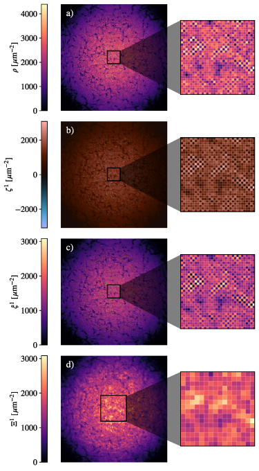
Figure 3. The first convolutional layer Conv1, elaborating in more detail the beginning of the image processing and feature extraction pipeline as depicted in figure 1. (a) Input of the atomic density, ρ. (b) Cross-correlation of the atomic density with the weights matrices (see equation (15)). (c) Application of the ReLU activation function and a bias (see equation (16)). (d) Carrying out maximum pooling (resulting in the halving of the image dimensions); this is one of j = 12 outputs of the first convolutional layer, as per equation (17). To the right we show zoomed-in sections of each step of the first convolutional layer as we construct the first layer feature maps.
Download figure:
Standard image High-resolution image
Layer 1: from a single input to 12 features
In the first layer ( ), we extract C1 = 12 features from the single input image ρ (such that the number of features in the ‘zeroth layer’ is C0 = 1). The weights for this layer consist of C1 = 12 filters connecting the single input channel (k = 1) to each output channel j, denoted as
  for
for  . Each filter (in this layer and in all subsequent layers) is a square matrix of dimension
  , and we initialise each weight element within these filters, independently, from a uniform distribution
  (the range of the probability distribution function depends on the number of features in the previous layer—see appendix
We carry out cross-correlations (see appendix  to compute the intermediate feature maps
  :
:

Here,  (assuming appropriate padding, see appendix
We then add a feature-map-specific bias term  (these are always drawn from the same distribution, appropriate to the layer, as the weights) to each matrix element of the intermediate feature map, and subsequently also apply the ReLU activation function to each element:

We show the activation function and bias applied to a single output of the cross-correlation in figure 3 c) (figure F2 in appendix  of adding the bias and applying ReLU activation to each of the intermediate feature maps
  ).
).
Finally, we apply MaxPool with a  window and stride 2 (see appendix
  :
:

This halves the matrix dimensions, so that  . These C1 = 12 feature maps
  , each of size
  , become the input to the next layer. We show a single, maximally pooled output in figure 3(d) (figure F3 in appendix
Layer 2: from 12 features to 24 features
In the second layer, we extract C2 = 24 features from the C1 = 12 input feature maps. The weights for this layer consist of  filters, denoted as
  for
for  (output channel index) and
  (input channel index). We initialise each weight element within these filters independently,
  .
.
We compute the intermediate feature maps  by summing the cross-correlations over all input channels:

See figure F4 in appendix  , followed by application of the ReLU activation function:

Figure F5 in appendix  :
:

The matrix dimensions again halve, so  . These C2 = 24 feature maps
  , each of size
  , become the input to the next layer; figure F6 in appendix
Layer 3: from 24 features to 48 features
In the third layer, we extract the final C3 = 48 features from the C2 = 24 input feature maps. These final features feed into the subsequent prediction pipeline. The weights for this layer consist of  filters, denoted as
  for
for  and
and  . We initialise each weight element within these filters independently
  .
.
We carry out cross-correlations, add bias terms, and apply the ReLU activation function and MaxPool (with stride 2) in exactly the same way as in the second layer. Hence,



Here,  . These C3 = 48 feature maps
  , each of size
  , are the final feature maps from the image processing and feature extraction pipeline that feed into the prediction pipeline, and can be seen in figure F9 in appendix
3.5. Computational considerations and learning
3.5.1. Cost function
Training a neural network involves optimising its parameters (the weights and biases) to minimise a cost function. For our model, which determines chemical potential and temperature, we consider the square error

When determining  , we express both the temperature and chemical potential in nanokelvin; with regard to
  and
and  , these values are strictly speaking chemical potentials divided by
  , and then expressed in nanokelvin. The values making up
  are thus comparable and of moderate magnitude.
3.5.2. Batching
For computational efficiency, we train the network using batches of atomic densities, each with independent associated temperature and chemical potential values, rather than processing them individually. We process input batches of size β (typically 16, 32, 64 or 128) as multidimensional arrays6, which we form by adding two additional channels, β and  , to the matrix at a given layer
  . The cost function with batching is

Weight matrices and bias terms in each convolutional layer are shared across all items in a batch, such that the same learned filters are applied identically to each input sample. This architectural choice does not reduce the number of parameters relative to processing individual inputs, but it avoids parameter duplication across the batch, thereby preserving model compactness and promoting generalisation. Moreover, while the data are different, because the operations applied to each sample are mathematically identical, the use of batches enables these computations to be vectorised and executed in parallel on GPU hardware. This leads to improved computational efficiency without altering the underlying functional form of the network. In practice, this parallelism is realised by arranging input data as multidimensional arrays with an added batch dimension, facilitating simultaneous convolution, activation, and pooling operations across multiple samples.
3.5.3. Training
To minimise the cost function in equation (25), we use the adaptive moment estimation (Adam) algorithm [37]—a widely used and generally effective adaptive learning rate method suitable for training large networks; see appendix D, section 4 of [34] for detailed derivations—using the default values for the learning rate, η = 0.001, and decay rates,  , and backpropagation for gradient calculation. We iteratively use Adam over 100 epochs—where each epoch processes the entire dataset in randomly selected batches (without replacement)—although we note a posteriori that using fewer epochs is possible since the cost saturates at around epoch 50, as shown in figure 5. After training, we save the learned weights and biases. Post-training, we can load these optimised parameters into a network with the same architecture to make rapid inferences from new data. We observe inference times for our model of the order of milliseconds in wall-clock time.
As described in section 3.4, in each layer the determination of the ζ matrices is associated with the introduction of the weights, and the determination of the ξ matrices with the introduction of the biases. Determination of the Ξ matrices is not part of the learning procedure, but processes the images for the next layer by halving the image dimensionality through MaxPool.
4.1. Interpretation of the feature maps
In figure 4 we show schematically the steps described mathematically in section 3.4 to produce from an initial density profile the feature maps from each of the three convolutional layers in the image processing and feature extraction pipeline. This displays subsets of the 12 feature maps produced in layer 1, the 24 feature maps produced in layer 2, and the 48 feature maps produced in layer 3, where plots, with colour axes, for the complete set of pre-activation images (the ζ matrices), post activation images (the ξ matrices), and feature maps (the Ξ matrices), for the same run, are displayed in appendix
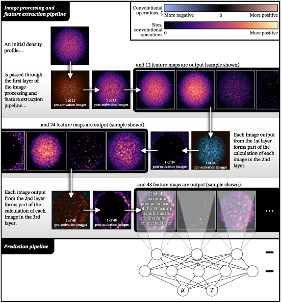
Figure 4. Schematic showing the production of the final 48 feature maps from an initial density profile, via the image processing and feature extraction pipeline, which then feed into the prediction pipeline (see also figure 2) to determine estimated values of the chemical potential µ and temperature T. The initial density profile is the same as that of figure 3(a), the (1 of 12) pre-activation image is the same as in figure 3(b), the following post-activation image is the same as in figure 3(c), and the first of the following sample from 12 feature maps is the same as in figure 3(d). Relative to figure 1, this schematic depicts detailed progress, a single channel of each layer at a time, through the image processing and feature extraction pipeline (see section 3.5.2 for details). The end-of-layer outputs from all channels (individual ‘slices’ in figure 1) are inputs to the subsequent layer; the 48 feature maps output by layer 3 are individually globally maximally pooled, as per section 3.3. The complete set of pre-activation images, post-activation images, and feature maps, for each layer, can be seen in in appendix
Download figure:
Standard image High-resolution image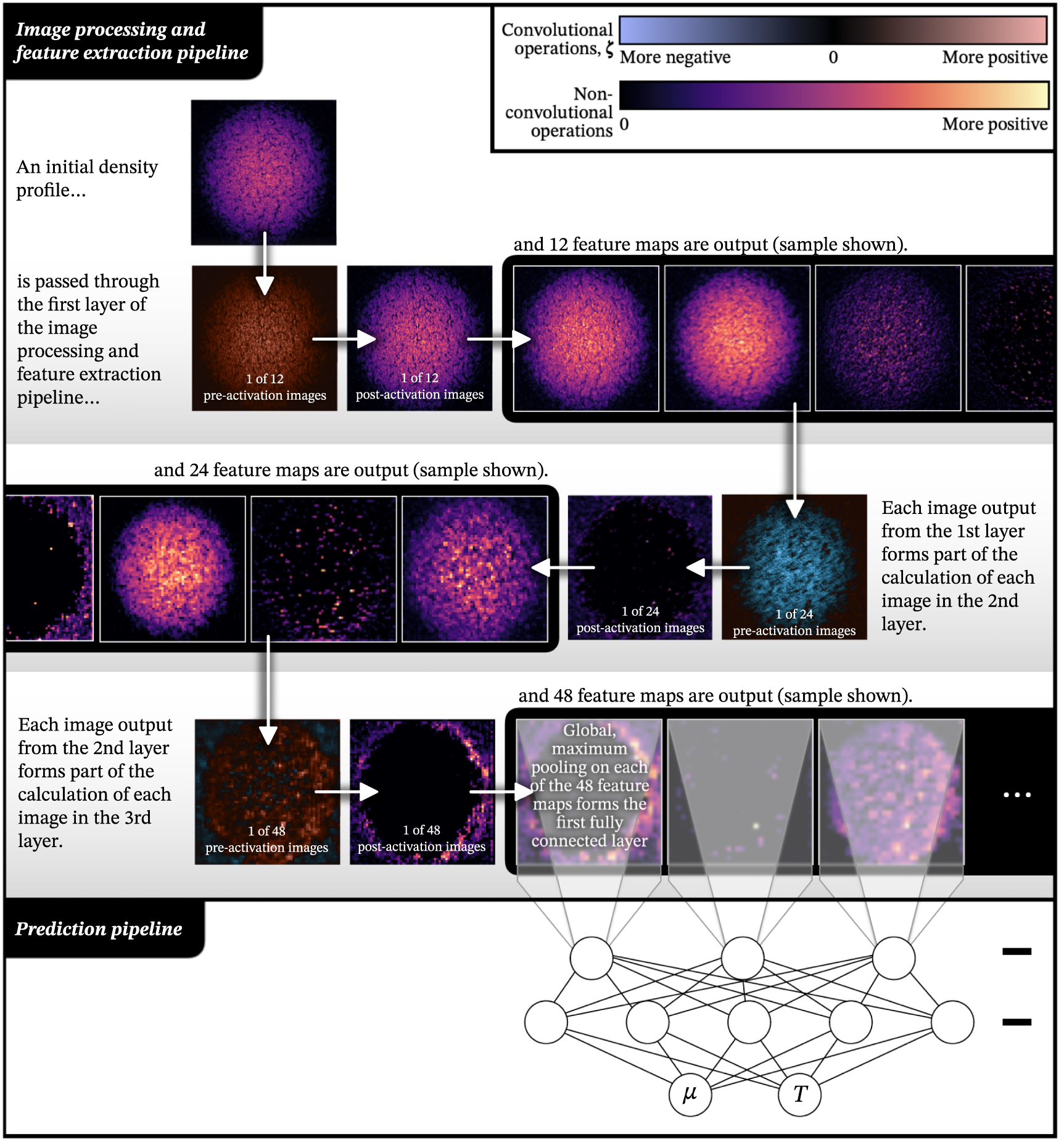
Increasingly abstract feature maps are learnt as we progress through the three layers. These features may include local variations in the density, patterns, or edges corresponding to the trapping potential, recognisable structures such as vortices, or other structures in the atomic cloud. The features may be local or global, with the convolutional layers trying to identify the fingerprints of the chemical potential and temperature values in the spatial structure of our input samples. The first set of feature maps, produced in the first convolutional layer (a subset of which are shown in figure 4), learn high-density features which we can reasonably infer to be associated with the chemical potential, since the chemical potential is fundamentally connected to the average atom number. For the complete set of pre-activation images, post activation images, and feature maps see appendix
Recognising the distinct roles that the chemical potential and temperature have in our feature maps, we design a series of interrogations to ascertain how our model could be used in a range of experimentally relevant protocols. In particular, we ask: 1) does the predictive capability of the model depend on whether the density profile being observed is at or very close to thermal equilibrium (which strictly speaking is required for the chemical potential and temperature to be properly defined), e.g. could we predict the chemical potential and temperature during the thermalisation of a condensate? 2) If the model does not have a strong dependence on the equilibrium distribution, could we use the model on toroidally trapped condensates? 3) Can our model predict the chemical potential and temperature of an ensemble average of equilibrium states? We will address each of these questions in turn, immediately after presenting our choice of model, which we do in the next section.
4.2. Model accuracy
We considered a balance of computational cost (models extracting more features per layer have higher computational cost) and model accuracy (using a metric which we refer to as the accuracy within 5%, as defined below) to determine which model to use in our subsequent analysis. We considered models with batch sizes of  or 128 (see section 3.5.2 for details), which extract either 6, 12 and 24 features, 12, 24 and 48 features or 16, 32 and 64 features in each convolutional layer.
Figure 5 shows the training and validation cost metrics for the models that extract 12, 24 and 48 features in the convolutional layers over a range of batch sizes. The absence of divergence between the training and validation cost metrics is often used as a heuristic to assess whether overfitting is occurring; in this case, it provides no such indication. Note that this figure alone is insufficient to ascertain the accuracy of the models. We observe no appreciable divergence in the training or validation cost metrics for all models (with fewer or more features)—all models approached final costs of the order of 10−1, despite their accuracy varying significantly.
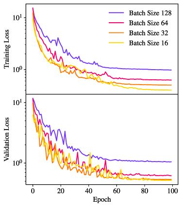
Figure 5. The training and validation cost metrics for batch sizes 16, 32, 64, and 128 from a model extracting 12, 24 and 48 features in the first, second, and third convolutional layers. A smaller batch size results in models with a lower overall training and validation cost.
Download figure:
Standard image High-resolution image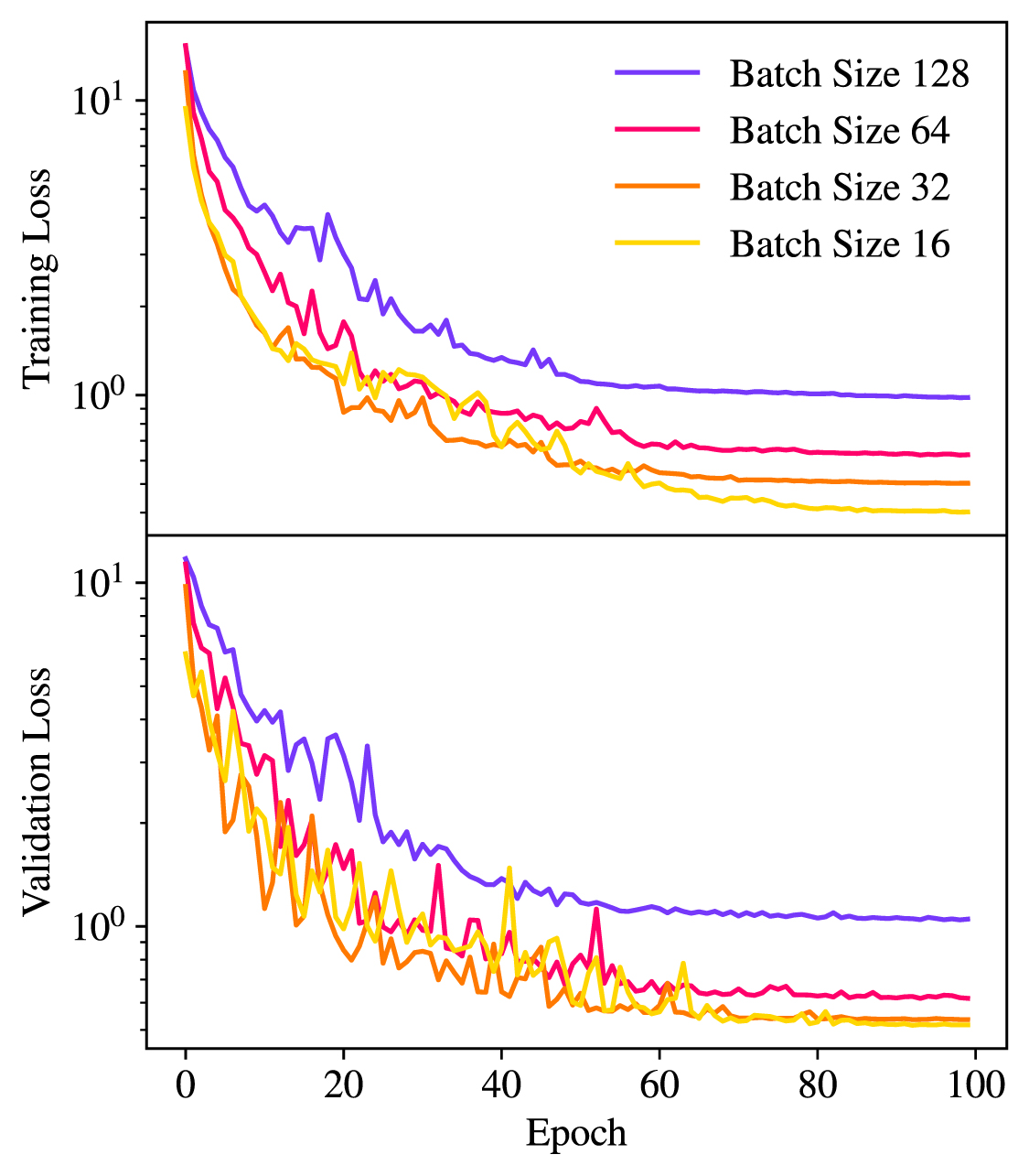
We define ‘accuracy within 5%’ as the proportion of samples with predictions within 5% of their true values—that is, the values which we set as input parameters to the stochastic evolution. Using this metric, figure 6 illustrates the predictive accuracy on the test dataset held back for this purpose, for models with 12, 24, and 48 convolutional features, across batch sizes  and 128. We see that the standard deviation of absolute errors decreases with decreasing batch size, indicating more accurate predictions of both chemical potential and temperature. Smaller batch sizes generally improve generalisation [38] by introducing more stochasticity into the optimisation process, helping the model escape shallow local minima and find solutions that generalise better to unseen data, and this is what we appear to be observing here.
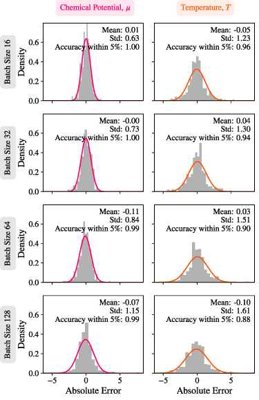
Figure 6. The histograms and corresponding normal distributions demonstrate the absolute error in the model’s prediction of the chemical potential (column 1) and temperature (column 2) of the held-out test data set to the true values input to our SGPE simulations. The plots share a common x-axis for easier comparison. These plots correspond to the models which extract 12, 24 and 48 features.
Download figure:
Standard image High-resolution image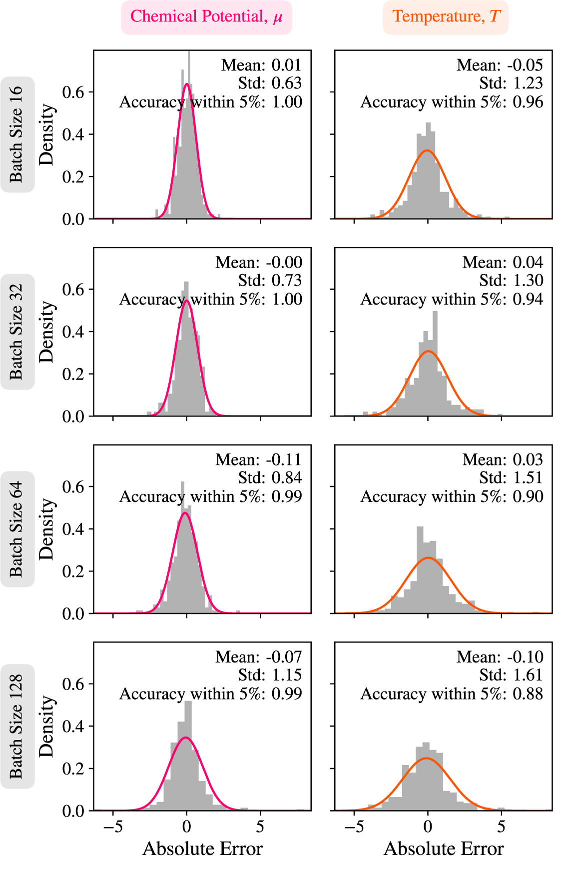
As summarised in table 1, reducing the convolutional feature set to 6, 12, and 24 features has negligible effect on chemical-potential estimation but degrades temperature prediction, whereas the 12, 24, and 48 feature configuration gives the best balance of speed and accuracy. Models with 16, 32, and 64 features produced no measurable improvement over the model with 12, 24, and 48 features—accuracies unchanged to two decimal places. We have found that the model that extracts 12, 24, and 48 features, with a batch size of 16, offers a good balance between speed and accuracy. All analyses from this point on use this model.
Table 1. Test dataset accuracy for chemical potential µ and temperature T, defined as the proportion of predictions within 5% of the true values (see § 4.2). Results shown for three model groups (feature sets) across batch sizes β. The models with the best accuracy within 5% for the chemical potential and temperature are highlighted in bold.
| Model (features) | Batch size β | Accuracy within 5% (µ) | Accuracy within 5% (T) |
|---|---|---|---|
| 6, 12, 24 | 16 | 1.00 | 0.92 |
| 32 | 0.99 | 0.92 | |
| 64 | 0.98 | 0.82 | |
| 128 | 0.98 | 0.73 | |
| 12, 24, 48 | 16 | 1.00 | 0.96 |
| 32 | 1.00 | 0.94 | |
| 64 | 0.99 | 0.90 | |
| 128 | 0.99 | 0.88 | |
| 16, 32, 64 | 16 | 1.00 | 0.96 |
| 32 | 1.00 | 0.94 | |
| 64 | 0.99 | 0.90 | |
| 128 | 0.99 | 0.88 | |
We briefly note that column-integrated 3D atomic densities may also be used in our model with similar accuracy to the quasi-2D condensates. Given a three dimensional atomic density profile,  , the column-integrated density (assuming the imaging is in the z-direction) is

The column-integrated density may then be passed through the machine learning model as previously described with no further post-processing.
4.3. Prediction capability and robustness
4.3.1. Estimation capability during thermalisation
In our simulations the bath, with which there is formally both heat and particle exchange, is consistently parametrised throughout by a constant chemical potential, µ, and temperature, T. We do not consider dynamics following any form of quench, and the machine learning model is trained only on thermalised Bose gases. As described in equation (9), we use convergence of the atom number as a practical criterion for having achieved thermal equilibrium. However we note that estimated values for µ and T given by our model appear to trend to the final values more quickly, during the thermalisation process and after a relatively brief transient, as shown in figure 7. During the initial stages of evolution (approximately  , as shown in figure 7), the model significantly underestimates both µ and T. At these early times, the atomic density distribution has not yet developed the equilibrium spatial features that the convolutional layers have learned to recognise: specifically, the Thomas–Fermi-like bulk profile that encodes µ through the overall density scale and spatial extent, and the statistical properties of thermal fluctuations that encode T. However, once these characteristic structural features begin to emerge—which occurs whilst the condensate atom number is still evolving toward the equilibrium value defined by our convergence criterion (equation (9))—the model’s predictions converge rapidly to accurate values. This demonstrates that the model has learned to extract features indicative of the system’s eventual thermodynamic state before full equilibration is achieved, despite training exclusively on equilibrium density profiles.
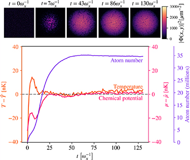
Figure 7. The evolution of the estimates of the chemical potential and temperature over the thermalisation procedure on dual axes. The pink line is the absolute error in the chemical potential. The orange line is the absolute error in the temperature. The purple line is the atom number. Top: evolution of a harmonically trapped condensate. The temperature of the same is 30 nK. The chemical potential of the sample is also 30 nK. The absolute errors in the temperature and chemical potential plateau after 80 units of rescaled time.
Download figure:
Standard image High-resolution image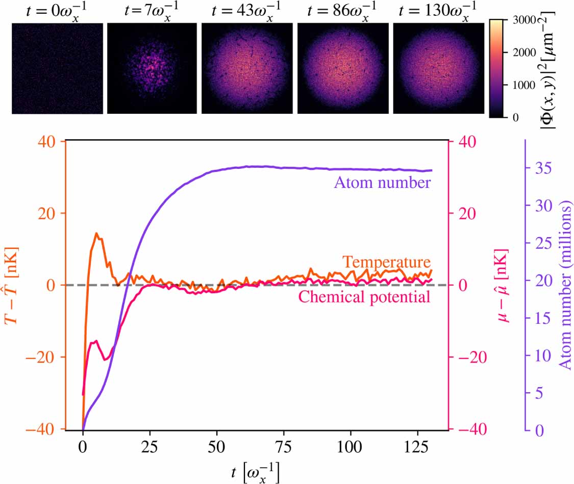
4.3.2. Toroidally trapped condensates
Toroidally trapped condensates permit metastable persistent currents (quantised flow of Bose–Einstein condensates in a multiply connected geometry) [39] and provide an appropriate geometry for experimental protocols such as weak links [40, 41] which are used in several atomtronic devices such as rotational sensors [10]. As an additional probe of the robustness of our model, which has been trained exclusively with harmonic trapping configurations, we apply it to toroidally trapped condensates. These have depth  , minor radius
  m and major radius
  m; we choose V0 such that
  .
.
While, as shown in figure 8, the estimated µ and T trend towards stationary values relatively quickly, the temperature is generally closer to the input value than the chemical potential. This difference reflects that µ is encoded in the bulk density distribution, which differs qualitatively between harmonic and toroidal traps, whereas T is encoded in small-scale fluctuations that are more geometry-invariant.
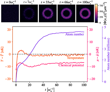
Figure 8. The evolution of the estimates of the chemical potential and temperature over the thermalisation procedure on dual axes. The pink line is the absolute error in the chemical potential. The orange line is the absolute error in the temperature. The purple line is the atom number. Top: evolution of a harmonically trapped condensate. The temperature of the same is 22 nK. The chemical potential of the sample is also 22 nK. The absolute errors in the temperature and chemical potential plateau after 80 units of rescaled time. The depth of the trap is 60 nK. The minor and major radii are, respectively, 20 µm and 40 µm.
Download figure:
Standard image High-resolution image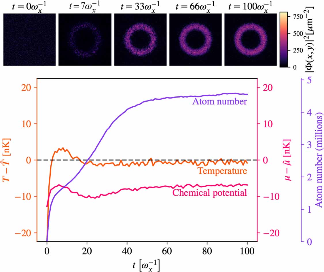
Convolutional neural networks exploit weight sharing—each  filter
  is applied identically across all spatial locations, so the same kernel contributes to every receptive field (i.e. each local
  patch of the input). During backpropagation, the gradient of a filter weight is accumulated over all receptive fields, so updating one weight modifies the response of that filter simultaneously at all positions. This enforces a translation-equivariant inductive bias [32], enabling the network to learn recurring local patterns independently of their absolute position. We interpret that convolutional filters scanning local receptive fields extract temperature-linked signatures that remain invariant under a change from harmonic to toroidal confinement.
Two additional factors accentuate the asymmetry: (i) the random transverse anisotropy injected during training (section 2.3) encourages robustness of local features to geometric perturbations, and (ii) the maximally global pooling before the fully connected layers discards absolute position, emphasising distributional summaries of fluctuation statistics rather than any geometry-specific structure.
4.3.3. Ensemble averages
Both average pooling and MaxPool are commonly used approaches in, e.g. image recognition. As discussed in appendix
As shown in figure 9, estimation of the chemical potential is quite comparable when using either maximum or average pooling, however when using average pooling information about the temperature is clearly lost. This is consistent with our observation, when considering toroidally trapped condensates, that estimation of the chemical potential is associated with the bulk distribution of the condensate (essentially similar regardless of the pooling type), whereas estimation of the temperature is associated with small-scale local density fluctuations, which will be averaged away by average pooling.
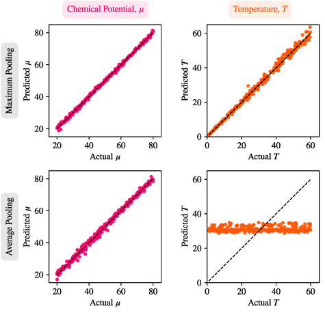
Figure 9. A comparison of the predictive capabilities of a network trained with maximum pooling and a network trained with average pooling. Both maximum pooling and average pooling are appropriate for learning and determining the chemical potential of Bose gases, but only maximum pooling is appropriate for learning and determining their temperature.
Download figure:
Standard image High-resolution image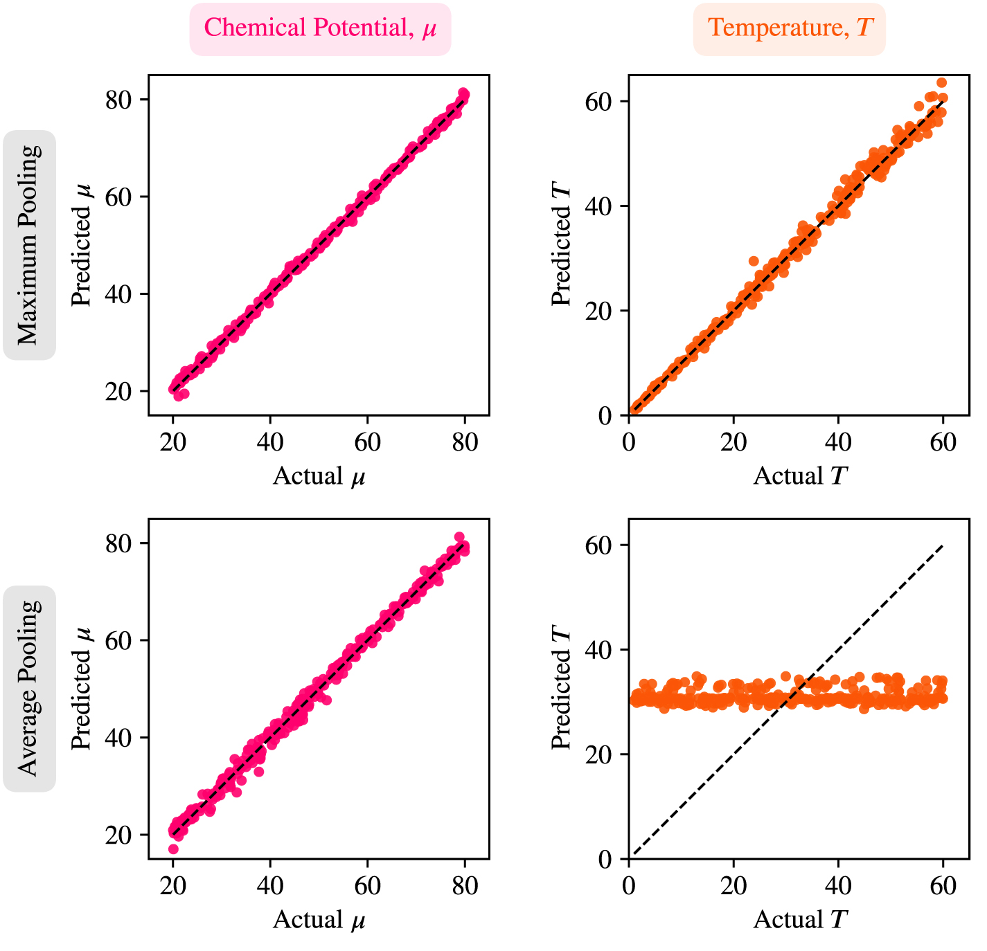
Similarly, as we have tested, averaging over many trajectories to produce an averaged density washes out the temperature-dependent background fluctuations, and we observe that ensemble averages passed through our machine learning model can only be used to obtain the chemical potential and not the temperature of the sample.
5.1. Effective pixel size
To establish an effective pixel size in a typical experiment, we consider the imaging system of Wilson, et al [45], which—like our model—considers in situ imaging of condensates to obtain position distributions. Wilson, et al use a Point Grey Firefly MV CMOS camera with pixels of size  m with a magnification of around 19.7, which leads to an effective pixel size of 6.0 µm/19.7 = 0.31 µm per pixel. We align our model’s theoretical maximum resolution to this effective pixel size based on this camera. For a quasi-2D ‘pancake’ condensate of diameter 80 µm in a harmonic trap, we need to use a grid size of
  in order to achieve an effective pixel size of about 0.31 µm.
5.2. Further considerations
Whilst our model’s resolution is appropriate for experimental data analysis, real BEC images often include additional complexities such as imaging artefacts, focus variations, and dark counts. In the work of Wilson et al, the optical resolution of the microscope (with a numerical aperture of 0.25) is actually diffraction-limited to  m when illuminated with light of wavelength 780 nm. More recent advances in in situ imaging of BECs by [46] and [47] report diffraction-limited resolutions of 0.7 µm and 0.9 µm, respectively. In practice this means that experimental images are effectively our simulated atomic density profiles convolved with the point-spread function of width given by the diffraction-limited resolution of the imaging system. Taking this known complexity into account—alongside augmentation with the other aforementioned experimental artefacts—would enhance the model’s robustness for real data. We also note that, while our model has been trained on in situ imaged position distributions, training on expanding time-of-flight velocity distributions is an in-principle straightforward extension, although significantly more demanding to generate if the full dynamics are included.
We also draw attention to very recent independent work, developed in parallel by De Sousa et al [48], for machine learning thermometry of a dilute, laser cooled (non-quantum-degenerate) vapour of potassium 39 atoms, from experimental data.
We have introduced a proof-of-principle machine learning model which can, with a single image, estimate the values of the chemical potential and temperature of a Bose-condensed cloud of atoms. We use convolutional neural networks—the foundation of most image recognition models—to take an atomic density profile and estimate important thermodynamic parameters. We have demonstrated that our model for a harmonically trapped condensate can estimate to some degree the chemical potential and temperature for systems that it has not previously been trained on, including during thermalisation, and on toroidally trapped condensates. This work joins recent applications of machine learning in the quantum fluids literature, such as the identification of topological defects such as vortices and solitons, and the reconstruction of vortex filaments [19–21].
We thank K E Wilson for insightful discussions about the experimental considerations of this work. We thank the EPSRC, Grant No. EP/T015241/1 and EP/T518001/1, for funding this project.
The data that support the findings of this study are openly available at the following URL/DOI: https://github.com/0jg/bec-ml-thermometry [31] and https://github.com/0jg/sgpe-rs [49]
In section 3.4, we introduced the cross-correlation function. We define the cross-correlation function (between y and w) as

Relative to the more generally known convolution operation, the cross-correlation operation is effectively a clockwise rotation of the kernel by 180∘. We extend equation (A.1) to matrices by introducing another index, σ,

The cross-correlation operation may be interpreted as a Frobenius inner product of a sub-matrix of  and the kernel,
  [50].
[50].
For historical and conventional reasons, it is the cross-correlation that is calculated in machine learning libraries such as PyTorch [51] and Tensorflow [52]—‘convolutional’ neural networks are a technical misnomer, but during training, convolutions and cross-correlations should converge on the same result.
Since most of the data we are interested in are 2D matrices, it is equation (A.2) that we use throughout this paper.
In a convolutional layer  (where
  ), we aim to extract
  features (output channels) from the
  features (input channels) provided by the previous layer (layer
  ). For the first layer (
 ), the input is the single map ρ, so C0 = 1.
To compute the jth output feature map (where  ), we use a set of weights (filters). Specifically, for each input feature map k (where
  ), there is a 2D filter
  of spatial size
  . For
. For  , k can only be 1, so the filters are
  . The collection of
  filters
  is used together (summing their individual cross-correlation results with corresponding input maps) to produce the jth intermediate output map
  .
.
We initialise each individual weight element  (where
  are spatial indices within the
  filter) independently from the uniform distribution [51]:

Here,  is the number of input channels (‘fan-in’ channels) to the layer, and
  is the spatial area of the filter. The term
  represents the total number of inputs that contribute to a single element in the output map before activation (the fan-in). We sample the biases
  from the same distribution U.
The total number of distinct weight matrices (filters), Nfilters, in a convolutional neural network with L layers is

The machine learning problem is to find the appropriate weights  and biases
  which optimise the mapping from the input data to the desired output.
To preserve the spatial dimensions of the feature maps during the cross-correlation operation (before pooling), we apply zero padding around the input feature maps of layer  . For a filter (kernel) of size
  , where kW is odd (e.g.
  as used in the main text), we add κ zeros to each side (top, bottom, left, right) of the input maps, where

For  , κ = 1. This ‘same’ padding ensures that the output of the cross-correlation,
  , has the same matrix dimensions as the input feature maps,
  , before pooling is applied.
Pooling operations reduce the spatial dimensions (width and height) of feature maps. This provides a degree of translation invariance and reduces the computational cost in subsequent layers. Pooling operates independently on each feature map. A pooling kernel of size  slides across the input map with a stride Σ. Common types are average pooling (AvgPool), which computes the mean of the values within the kernel window, and MaxPool, which takes the maximum value.
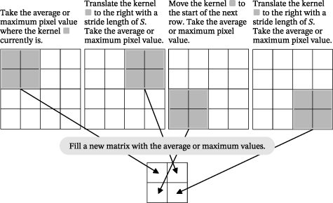
Figure D1. Illustration of pooling using a kernel of size  and stride length
  on a
on a  grid. The output is a square matrix with reduced width and height
  . In the main text, we use MaxPool with
  and
and  . The convolutional filters have size
  .
.
Download figure:
Standard image High-resolution image
In this paper, we apply MaxPool after the activation function in each convolutional layer ( ). The inputs to the pooling operation are the activated feature maps
  . We use a pooling kernel size
  and a stride
  . If an input map has matrix dimensions
  , the output map dimensions
  are given by:

For  , this simplifies to
  .
.
The output feature maps after pooling in layer  , denoted
  , are computed from the activated maps
  . Using
  for the output map,
  for the input map
  ), the MaxPool operation is:

With  and
and  , this matches the formulae used in the main text, e.g. equation (17).
The average pooling equivalent (not used in the main text) would be:

For conceptual comparison, we can draw an analogy between the operations in a convolutional layer (without pooling) and a fully connected neural network layer. Consider a simplified 1D case, where the output  of neuron j in layer
  of a fully connected neural network is typically computed as:


Here,  is the activation function,
  is the pre-activation value,
  are the activations from the previous layer (
 ),
),  is the weight connecting input neuron k to output neuron j,
  is the bias for neuron j, and
  is the number of neurons in layer
  .
.
In the convolution neural network context (equations (18) and (19)), ignoring pooling and 2D structure for simplicity), the computation for the jth feature map involves:


The key difference lies in equation (E.2b) using a local cross-correlation ( ) operation with shared weights within the filter
  , rather than a simple weighted sum (dot product) over the entire previous layer output as in equation (E.1b). However, both involve a form of weighted summation over inputs from the previous layer (summing over index k up to the number of input features/neurons,
  or
or  ), followed by a bias and activation function, highlighting the conceptual link.
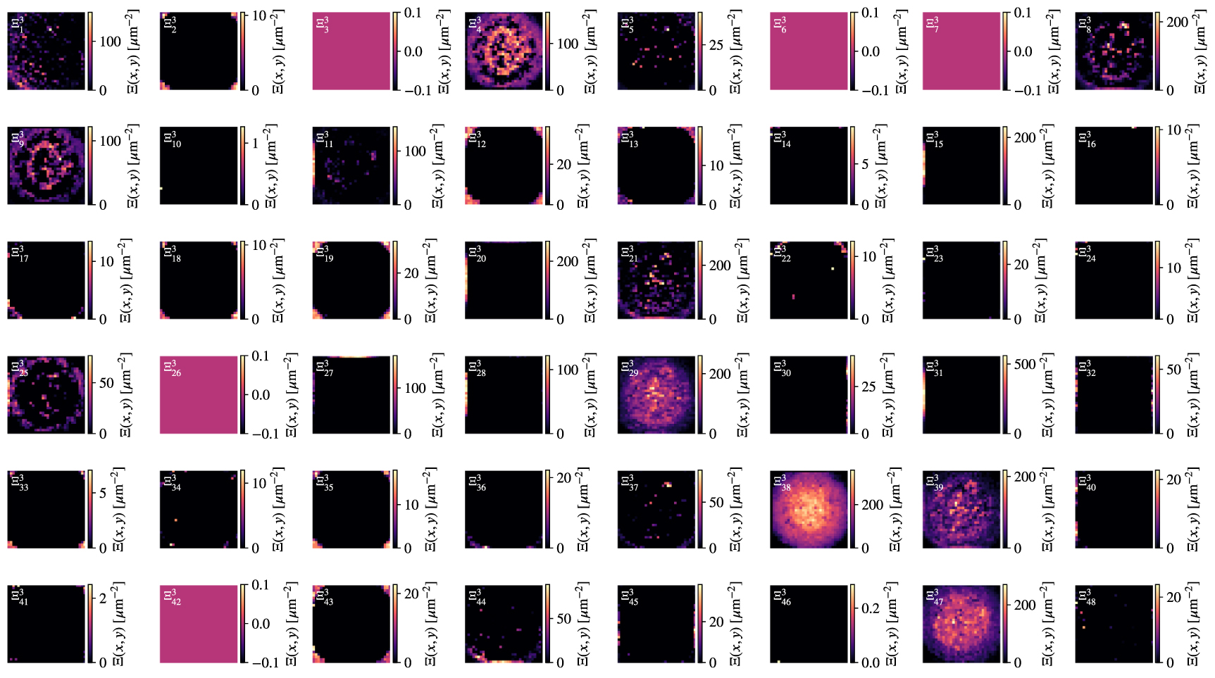
The figures in this appendix show the complete feature extraction process for the same atomic density profile used in figure 3. Each set of three figures corresponds to one convolutional layer: pre-activation maps (cross-correlation outputs), post-activation maps (after ReLU and bias), and final feature maps (after MaxPool).
Figures F1–F3 show the first layer outputs (12 features), which primarily capture high-density regions and large-scale structural information. Figures F4–F6 show the second layer outputs (24 features), which learn intermediate-scale patterns. Figures F7–F9 show the third layer outputs (48 features), which are sensitive to fine-scale fluctuations that encode temperature information.
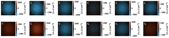
Figure F1. The cross-correlation, ζ1, of a single image of an atomic density,  , with 12 weights kernels,
  ,
,  , as determined by equation (15). The cross-correlation may result in positive or negative values, as indicated by the colour bars.
Download figure:
Standard image High-resolution image
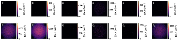
Figure F2. ξ1, the result of applying an activation function as determined by equation (16).
Download figure:
Standard image High-resolution image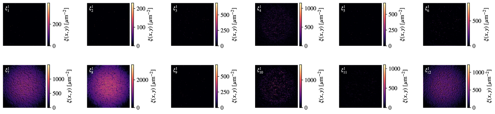
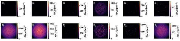
Figure F3. The maximally pooled features, and therefore the output of the first convolutional layer, Ξ1, as determined by equation (17).
Download figure:
Standard image High-resolution image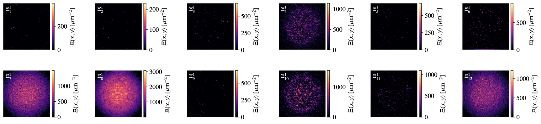
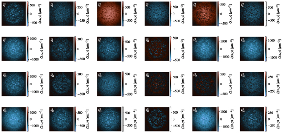
Figure F4. The cross-correlation, ζ2, of the features extracted from the previous layer, Ξ1, with 24 weights kernels,  ,
,  , as determined by equation (18). The cross-correlation may result in positive or negative values, as indicated by the colour bars.
Download figure:
Standard image High-resolution image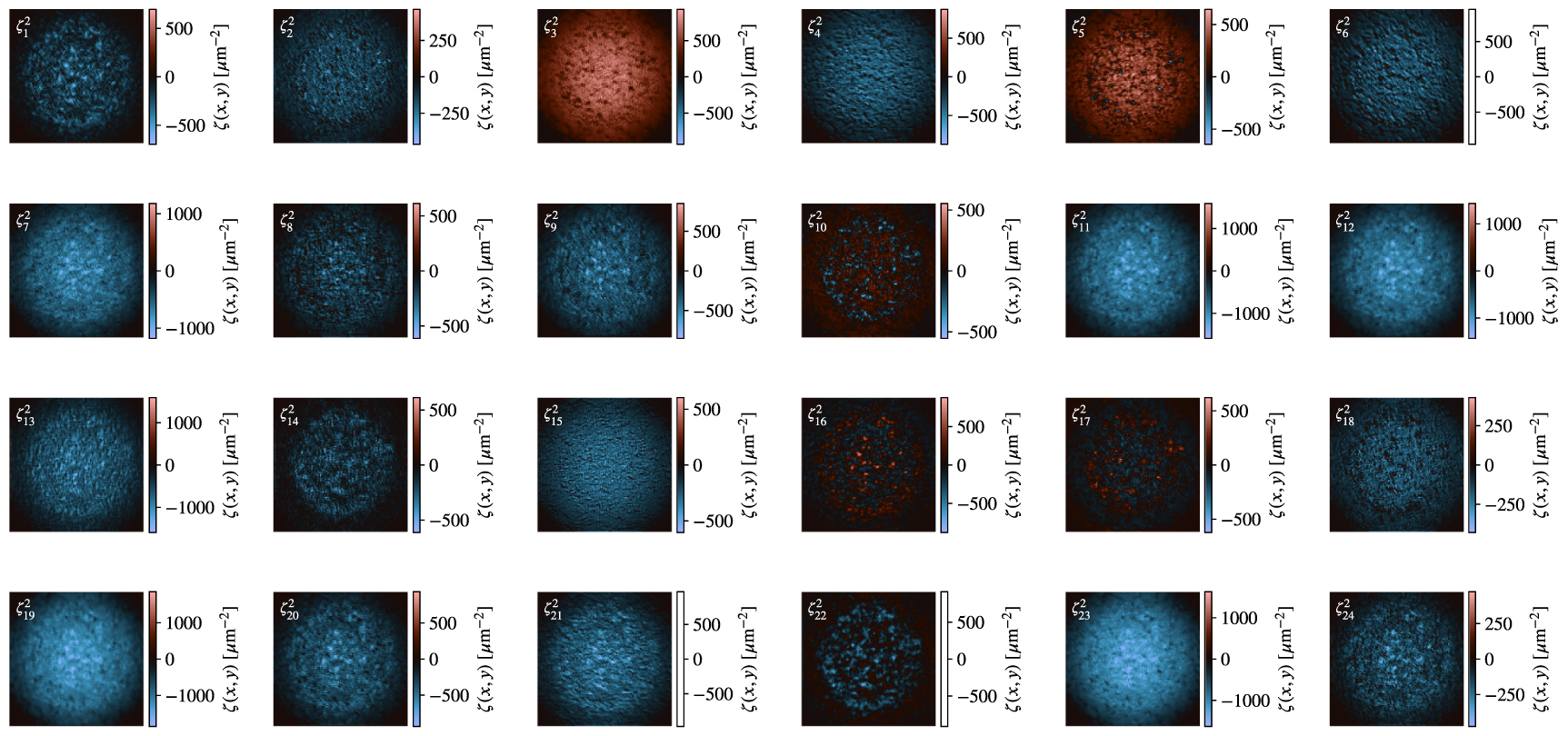
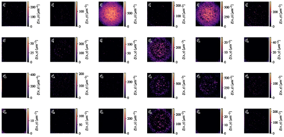
Figure F5. The post-activations, ξ2, as determined by equation (19).
Download figure:
Standard image High-resolution image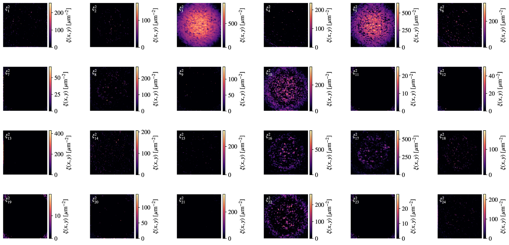
Figure F6. The maximally pooled features, and therefore the second layer outputs, Ξ2, as determined by equation (20).
Download figure:
Standard image High-resolution image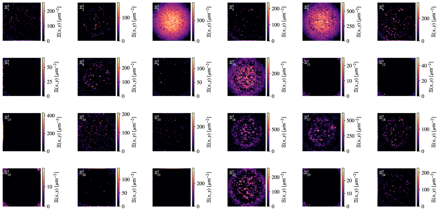
Figure F7. The cross-correlation, ζ3, of the features extracted from the previous layer, Ξ2, with 48 weights kernels,  ,
,  , as determined by equation (21). The cross-correlation may result in positive or negative values, as indicated by the colour bars.
Download figure:
Standard image High-resolution image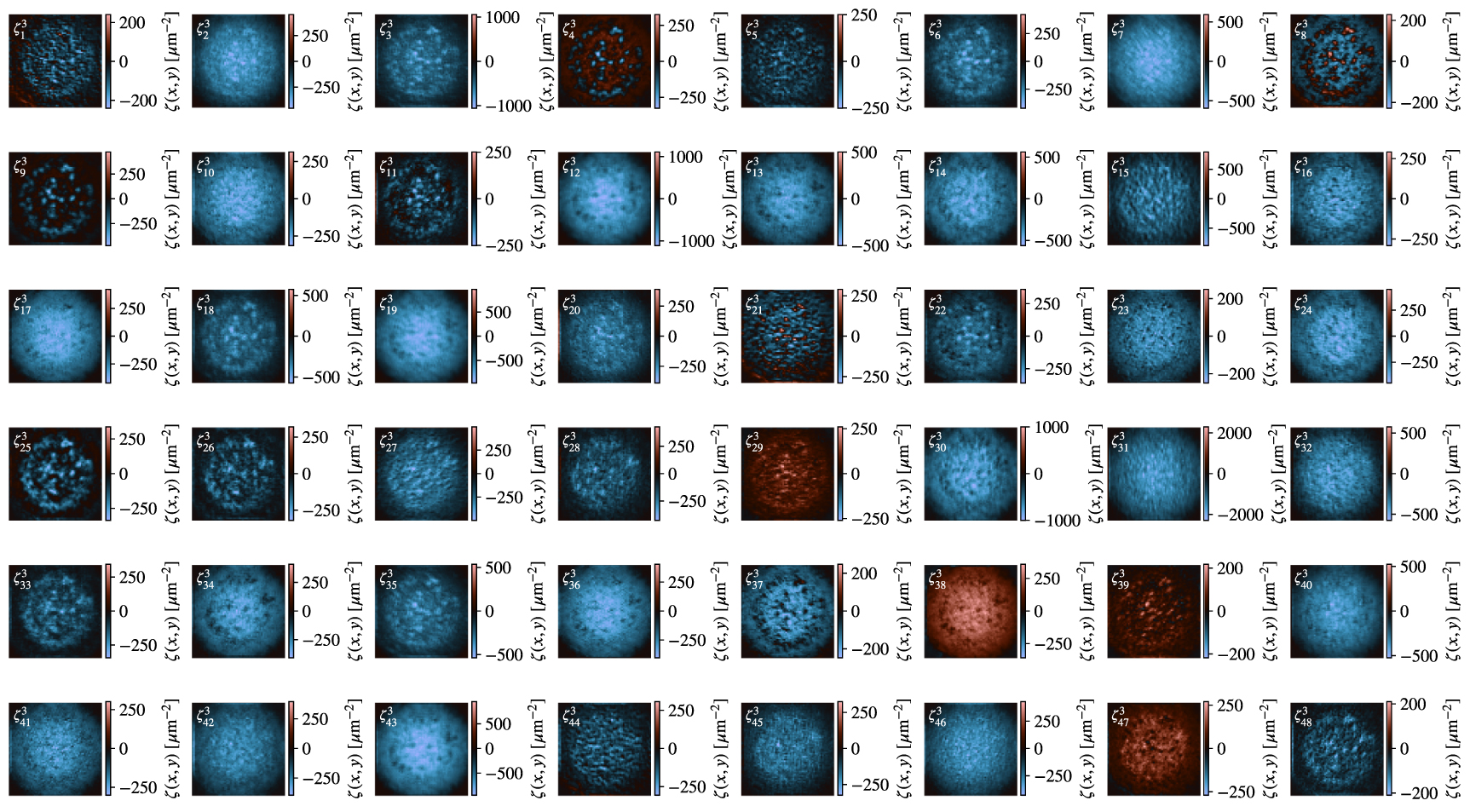
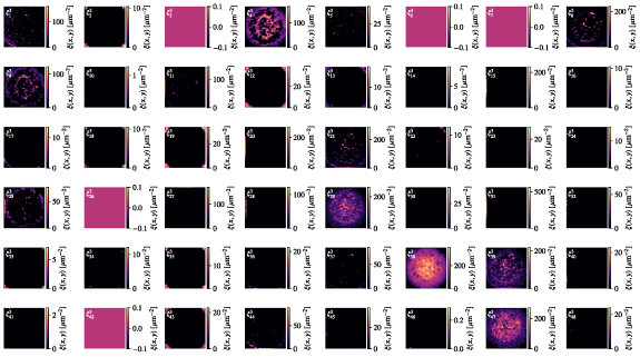
Figure F8. The post-activations, ξ3, as determined by equation (22).
Download figure:
Standard image High-resolution image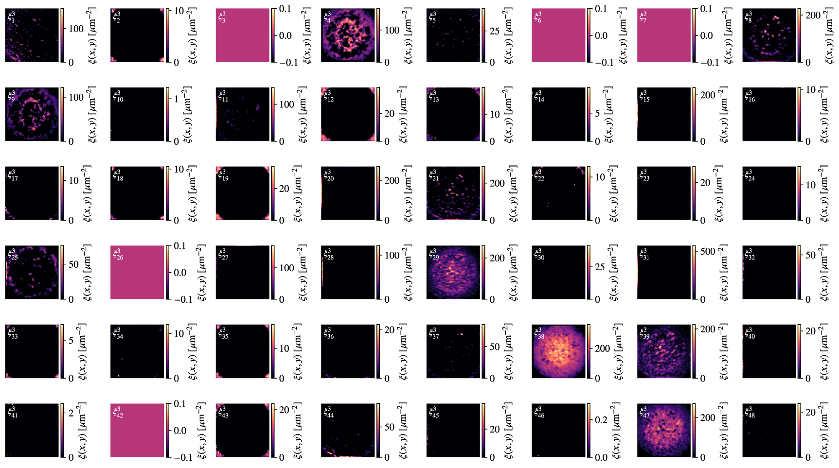
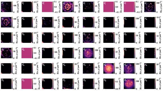
Figure F9. The maximally pooled features, and therefore the final output of the image processing pipeline, Ξ3, as determined by equation (23).
Download figure:
Standard image High-resolution image