GitHub - Neighborhood-Grid/flatpoints: Apply the principles of geometry images (https://hhoppe.com/proj/gim/) directly to point clouds. Each 3d point of the cloud become a 2d pixel, the pixels together form an image like indexing structure.

Turn a 3D point cloud sampled on a latent (unknown) surface into something flat.

INPUT: raw point cloud	OUTPUT: flat transformation

▶️ bunny 🐇
▶️ dragon🐉
▶️ elephant 🐘

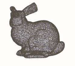flatpoints takes a raw point cloud (N, 3) and arranges its points on a square (n, n) grid of pixels:

• one pixel per point: each point gets its own pixel.
  idx -> (row, column)
• neighbour pixels hold neighbour points: two adjacent pixels hold two points close on the surface, so the image is a continuous picture of the surface.

Any data attached to the points, (N, *C), then becomes an image (n, n, *C): the xyz coordinates, normals, colours, features... and the whole 2D toolbox applies to the point cloud: convolutions and CNNs, SVD, grid interpolation…

This is the idea of the geometry images of Gu, Gortler & Hoppe (2002), which remesh a surface onto a completely regular grid. flatpoints applies it directly to a point cloud. How it works: see Method.md.

Install

pip install flatpoints                # core: numpy, scipy, gridpoints, open3d
pip install "flatpoints[viz]"         # + matplotlib, Pillow (plots, animations)
pip install "flatpoints[compress]"    # + PyWavelets, Pillow (compression)
#or pip install "flatpoints[all]"     # (everything)

Quickstart

Take a raw 3D point cloud (N, 3) and turn it into images. Available models: bunny, dragon, elephant, airplane, cow, everest… (fp.datasets())

import flatpoints as fp
fp.exemple_flat("bunny")   # prints the shapes, plots the surface and its images
fp.exemple_flat("bunny", save="plots", animate=True)  # + saves plots/bunny.png and plots/animation/bunny.webp

Usage

import numpy as np
import flatpoints as fp

xyz = fp.load("bunny") #raw (N, 3) points, on a latent (unknown) surface
z = xyz[:, -1] #(N, *C) any data related to the point cloud, e.g. the z coordinate

# ==== Build the flat object ============

flat = fp.Flat(xyz) # Apply the flattening processing of the surface
# flat = fp.Flat(xyz, mesh=(vertices, triangles))  # giving your mesh as additional input (optional).

# ==== Use it: pixels and images ========

i = 42 #point with index 42 (xyz[42])
face, row, col = flat.pixels[i] # face: 0 or 1 (see the Cut section)
image_z = flat.to_image(z)    # full pixel image,  (N, *C) to  (1, n, n, *C) or (2, n, n, *C)
fig = flat.plot()           # the surface in 3D and its images 
fig = flat.imshow(z)        # plot any data on the images
anim = flat.imshow(z, animate="z.webp") # animated version

Cut

To map the surface properly to a square, flatpoints need to cut it first in two hemispheres
if needed. The hemispheric cut will remove some (not all) topological closedness. Residual
closedness (e.g. for a torus, which cannot be opened by a single cut) will also be automatically
cut by shearing the surface further on each hemisphere.

• Use fp.Flat(points, single_face=True) for an open surface (e.g. a terrain),
  to flatten it on a single image.
• Use fp.Flat(points, single_face=False) for a closed surface (e.g. a dragon),
  to flatten left and right hemispheres independently, on two images.

One can specify a normal_axis (fp.Flat(points, single_face=..., normal_axis = "x")) to control which axis the surface is seen along. With single_face = False (two hemispheres), the surface is cut roughly across it. Any given normal axis will work properly, but it will result in a different cut. With single_face = True (open surface), the normal axis will only be used to orient the image (which way is up, where the corners go).

See fp.exemple_flat (examples.py).

Application: resampling a point cloud

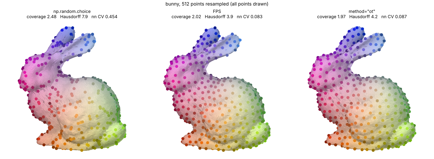
fp.exemple_sampler("bunny", save="plots")      # plots/resampling/bunny_resampled.png

Sampling from a mesh is easy: sample uniformly on each triangle. Resampling from a point cloud is harder, because there is no surface to sample from, only points.

The images provide that missing surface: to_image(xyz) maps the unit square onto the cloud. So one can sample points in the unit square and transport them onto the surface by bilinear interpolation of the xyz image, (row, col) → xyz.

By default, flat.resample uses a hyperuniform 2D seed (blue noise), so the new points are fairly evenly spread over the surface. If method = "ot" is used, the initial resampling is optimised further using Optimal Transport.

sampler = flat.resample(n_points=512, method="ot")   # n new points in total
new = sampler.points                    # (512, 3)
sampler.plot()                          # before / after

To be honest: if you only need a subset of the input points, farthest point sampling (FPS) is roughly as uniform as flatpoints (fps has slightly smaller worst case hole and flatpoints.resample slitghly lower ot loss), this is mainly an example usecase to show how to use the images to transport properties like good spatial repartition from the simple unit square to an arbitrary surface.

Application: compressing a point cloud

needs PyWavelets and Pillow (pip install "flatpoints[compress]")

fp.exemple_compression("bunny", save="plots")  # plots/compression/bunny.png

Since neighbour pixels hold neighbour points, the xyz images are smooth, and smooth images compress well. flat.compress compresses them with one of three methods (compressor.py):

• "svd": truncated SVD
• "dct": 2D DCT
• "wavelet": 2D wavelets

factor is the fraction of the storage saved against the points in float32 (96 bits per point).

comp = flat.compress(factor=0.8)  # save 80% of the storage, best method
comp.method                       # "dct"
comp.code                         # what is stored, e.g. quantized DCT coefficients and step
comp.points                       # (N, 3) reconstructed points, in the input order
flat.compress(0.8, method="svd")  # a given method
comp.save("compressed.jp2")       #save the compressed structure
points = fp.Compressor.read("compressed.jp2") #reconstructed (N, 3) point cloud

Licence

• code: MIT, except src/flatpoints/rcm.py.
• src/flatpoints/rcm.py: Python port (modified) of garyptchoi/rectangular-conformal-map, Copyright (c) 2015-2024 Gary Pui-Tung Choi, Apache License 2.0, see LICENSE-rectangular-conformal-map.
• src/flatpoints/data/seed.npy (shipped in the package): hyperuniform point cloud from the Hyperuniform samples database, MIT licence.
• example point clouds (data/, downloaded by fp.load, not shipped in the package): third-party models, each under its own terms (some research / non-commercial only), see data/README.md.

Acknowledgement

The concept of a surface stored as a square image comes from the geometry images:

@article{gu2002geometry,
  title   = {Geometry Images},
  author  = {Gu, Xianfeng and Gortler, Steven J. and Hoppe, Hugues},
  journal = {ACM Transactions on Graphics (SIGGRAPH)},
  volume  = {21},
  number  = {3},
  pages   = {355--361},
  year    = {2002},
  doi     = {10.1145/566654.566589}
}

The images rely on the rectangular conformal map of:

@article{meng2016tempo,
  title   = {{TEMPO}: Feature-Endowed {T}eichm{\"u}ller Extremal Mappings of Point Clouds},
  author  = {Meng, Ting Wei and Choi, Gary Pui-Tung and Lui, Lok Ming},
  journal = {SIAM Journal on Imaging Sciences},
  volume  = {9},
  number  = {4},
  pages   = {1922--1962},
  year    = {2016},
  doi     = {10.1137/15M1049117}
}