Note: FLOPS & Finance is going to be part of a series analyzing the economics of serving and training large models. It’s my own attempt at actually trying to build an understanding compute capacity planning, a field that is still relatively new, but one that a lot more tech companies will have to go through.

Image generated with Flux 2 (Just released so why not)
Heavily inspired by Piotr Mazurek and Felix Gabriel piece on LLM inference from first principles, this analysis will aim to achieve similar insights but for image generation models. In particular, we’ll be focusing on FLUX 1. Kontext [Dev], the first model to be able to do both image generation and image editing in one model. There has been a lot of analysis on inference cost for language models, but a lot less material on the economics of image generation. As to why inference cost matter, Tensor Economics has put it quite eloquently:
”For AI labs, token production costs fundamentally determine profit margins and the cost of generating synthetic training data-more efficient inference means higher returns on a fixed investment in hardware that can fuel further research and development cycles. For users, lower token costs democratize access to these powerful tools, potentially transforming AI from a premium resource into an everyday utility available for even routine tasks. Understanding these cost structures isn’t merely academic-it provides insight into one of the key economic forces that will shape AI development in the coming years as we approach increasingly capable systems.”
The implications for image generation differ from typical text generation workflows due to the significantly higher token count and compute intensity required for images. One interesting fact I’ve noticed in workflows for image generation is that people generate images in batches of 4 as default, leading to increasing costs.
For a quick primer, FLUX.1 Kontext [dev] is a 12B-parameter rectified flow Transformer implementing a Multimodal Diffusion Transformer (MMDiT) architecture. Although FLUX.1 uses a diffusion-like generative process, it was refined via Flow Matching and Latent Diffusion Distillation to minimize the number of steps needed.
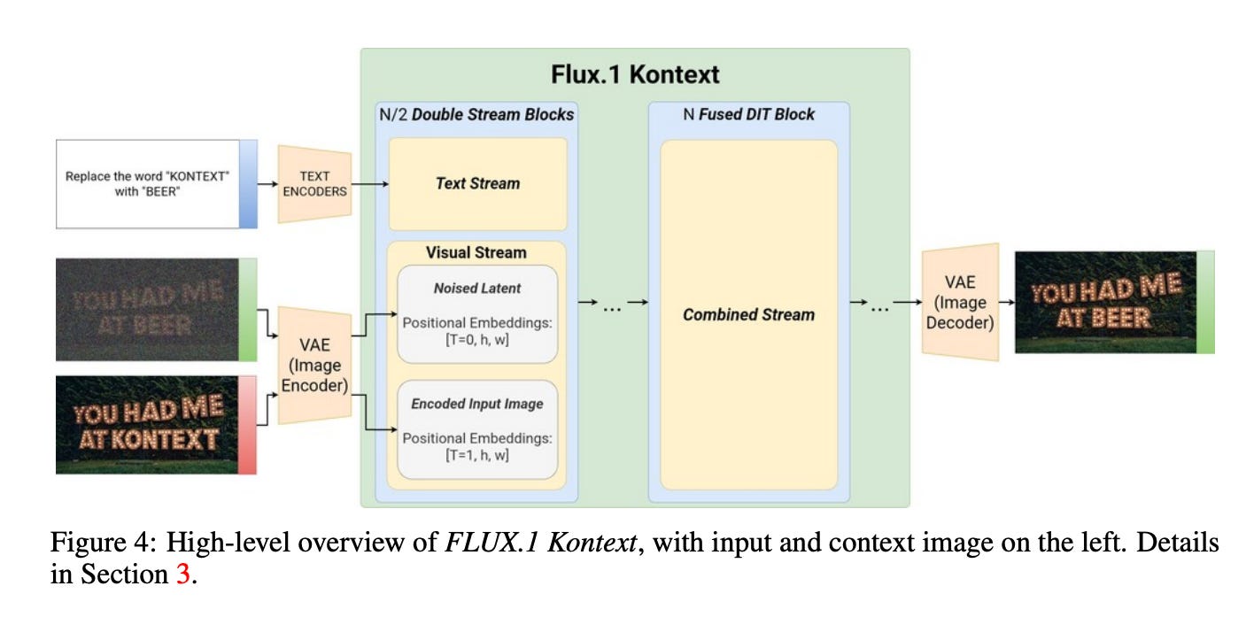
In standard diffusion models, generating an image might require 50–100 iterative denoising steps, each involving a forward pass of the U-Net model. FLUX.1’s approach means it can generate images in far fewer steps. I recommend watching the video on diffusion vs flow matching by AI Coffee Break with Letitia for explanation as to the efficiency gains. Each step is essentially one full forward-pass of the 12B parameter Transformer on the combined sequence of tokens (context + the image latent at a given timestep).
One caveat worth mentioning is in practicality, you want to calculate the actual inference cost from experimentation, meaning to look at how much time it takes to generate images and measure against cost per hour for GPU. This is because there are a lot of additional calculations and memory considerations that would be difficult to capture.
Aside from that, the calculations below are fully just estimates, and we will be making a lot of assumptions including:
Dense attention assumed: I’m assuming full attention over all tokens, but real models often use tricks that cut the compute down.
Perfect GPU usage assumed: The math assumes the GPU runs at peak speed, which rarely happens in practice.
Model optimizations ignored: Models use things like FlashAttention and mixed precision that change the actual FLOPs.
Extra overhead not counted: VAE steps, text encoding, and other non-compute tasks add time that isn’t included here.
For our set up, we will assume a few things:
We will be running on H100
We want to generate a 1024x1024 image
We will be passing through 100 tokens in text as prompt sequence
We will be running 10 steps/passes for image generation
We will only be calculating for the text to image process (Possibly will run separate calculations in another post for image editing)
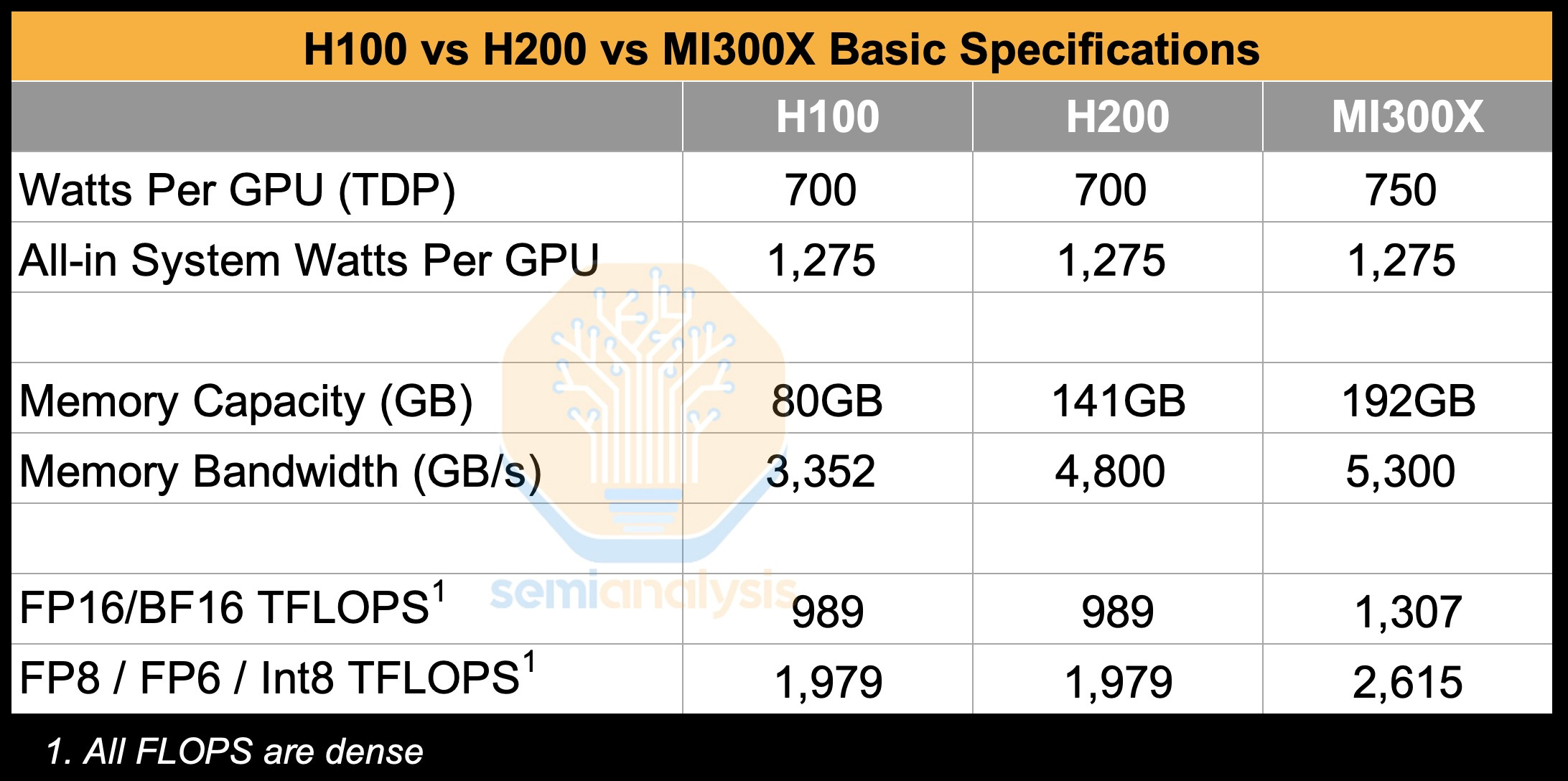
The model size for FLUX.1 Kontext being 12B parameters and being stored in BF16 then the size of the model would be around 24 billion bytes or 24GB, which fits well within 1 H100. Based on SemiAnalysis benchmark report of the H100 these are the expected specs:
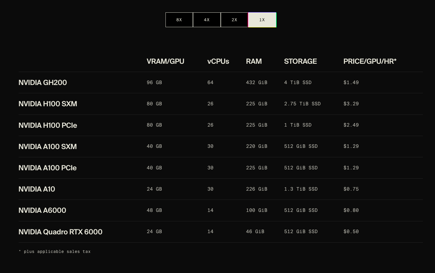
We can also find the cost of a H100 by looking at providers such as Lambda prices an instance of NVDIA H100 SXM at $3.29 an hour.
For inferencing the FLUX.1 Kontext model, we can find the information from the official repo on inferencing. Here we can see that the key steps are:
Noise Generation
Context Encoding (Text Prompt Embedding)
Flow Sampling (Denoising)
Latent-to-Image Decoding (VAE)
In layman terms, FLUX starts by creating a field of random noise. Your text prompt is then encoded into a numerical form the model can understand. The model gradually transforms the noise into a coherent image by running several “flow” steps, each one nudging the noise closer to what the prompt describes. This produces a lower-resolution latent image, which is then decoded and upscaled back into a full 1024×1024 image.
We will skip over noise generation, context decoding and VAE decoding as the number of FLOPs is trivial in comparison to the actual attention blocks. However, I highly recommend on your own time going over it if you are interested, as there are a lot of things to learn.
For estimating FLOPS per matrix multiplication, we will borrow the term from Tensor Economics:
Total FLOPs = (2n-1) × m × o ≈ 2mno
where m, n and o come from
When multiplying matrices A (shape m×n) and B (shape n×o), we produce matrix C = A @ B (shape m×o).
Full explanation can be found here
Probably the most exciting part and challenging part to uncover for FLOPs. To calculate the FLOPs here we need to understand what happens when we do a pass through in a multi model diffusional transform. FLUX.1 model specifically uses a variant of MMDIT with 57 layers in total, 19 dual branch blocks and 38 single branch blocks. The idea here is to process I want to give a quick shoutout to SNU for their phenomenal paper Exploring Multimodal Diffusion Transformers for Enhanced Prompt-based Image Editing which goes into good detail about the attention mechanism for the model.
For simplicity’s sake we will skip over the activation function FLOPs, RoPE and rectified flow update as they take up almost no FLOPs in comparison to the pass through. However Tensor Economics covered quite clearly in their LLM inference economics essay on RoPE in case you are interested.
There is also one BIG caveat I must address, for explainability and brevity I will treat the single and double stream block as single stream input. In practice for accuracy you should probably calculate them separately, as in run the input sequences separately but for explainability purposes we will treat them as one. Double stream blocks process text and image separately while single stream blocks are applied later and fuse the two inputs.
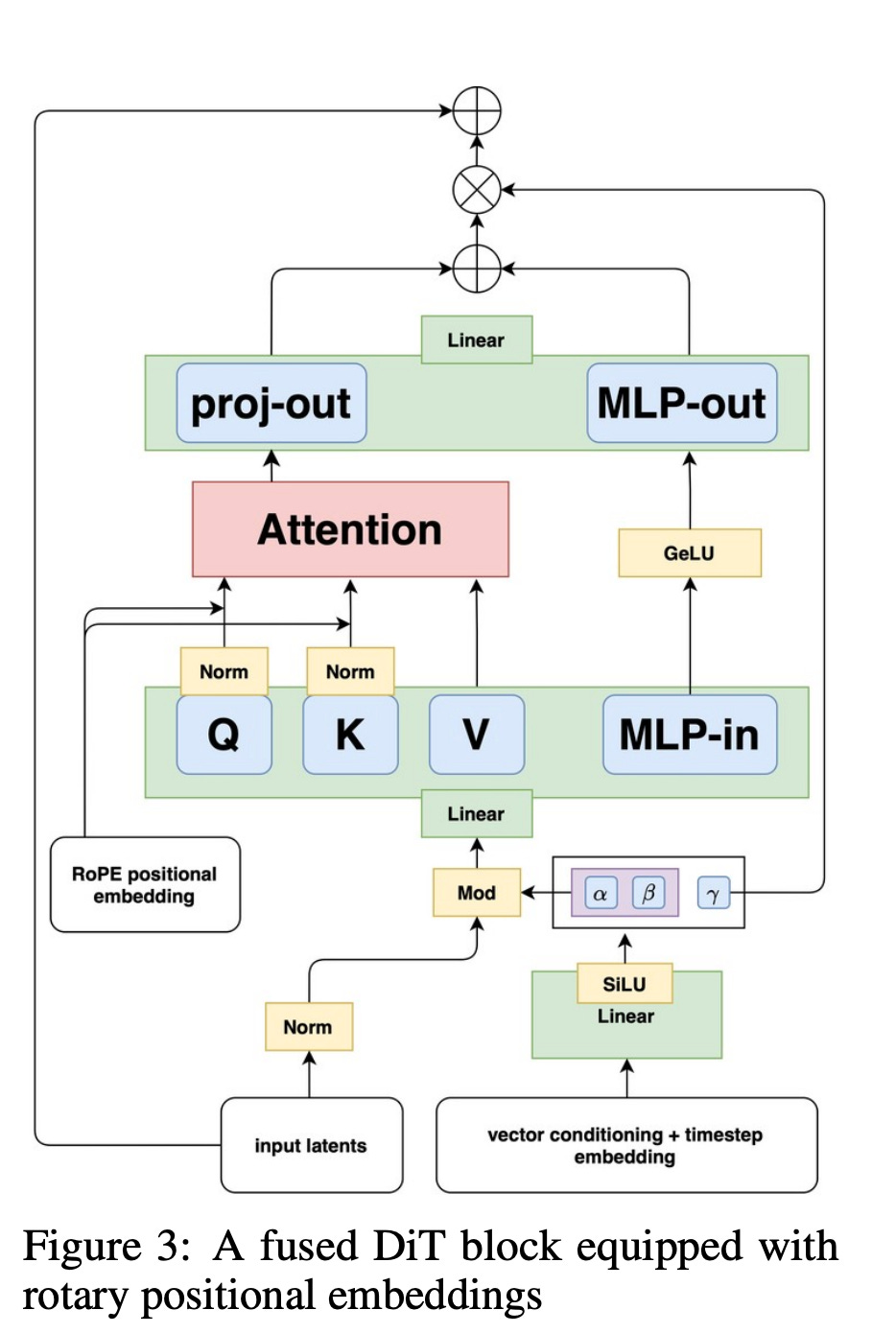
For the FLOPs calculation of the DiT blocks, we basically need to calculate three components:
Query, Key and Value Projection
Attention Mechanism
Feed Forward through MLP
Here will be our variables based on the official documentation, our assumptions earlier and what I’ve gathered:
Text Token Size = 100
Image Size = 1024 × 1024
VAE downsample factor r = 8 → latent grid 128 ×128
Sequence Size = 128 × 128 + 100 = 16484
Number of heads: 24
Head dimensions: 64
Flux hidden size d=1536
For the formulas this time, rather than doing our own calculations like above we can borrow from Tensor Economics in their LLM inference economics paper which is as follows:
\( \mathrm{FLOPs}_{Q} = 2 \, S \, d^{2} = 2 \cdot 16484 \cdot 1536^{2} ≈ 7.7\cdot 10^{10} \)
Similarly, we can borrow from Tensor Economics to get the Key and Value, the difference though compared to their formula is we don’t divide by 8 as FLUX 1 does not use multi head grouped attention query.
\( \mathrm{FLOPs}_{K+V} = 4 \, S \, d^{2} = 4 \cdot 16484 \cdot 1536^{2} ≈ 1.56 \cdot 10^{11} \)
We will also assume a naive implementation rather than using flash attention for our calculation.
\( \mathrm{FLOPs}_{\text{attn}} = 2 S^{2} d_{\text{head}} H = 2 S^{2} d = 2 \cdot (16484)^{2} \cdot 1536. ≈ 8.35 \cdot 10^{11}\)
Here we will make the same assumption for FLOP estimation. H here is number of attention heads.
\( \mathrm{FLOPs}_{\text{softmax}} = 5 S^{2} H = 5 \cdot (16484)^{2} \cdot 24 . ≈ 3.26 \cdot 10^{10} \)
\(\mathrm{FLOPs}_{\text{attn-out}} = 2 S^{2} d = 2 \cdot (16484)^{2} \cdot 1536 ≈8.36×10^{11} \)
\(\mathrm{FLOPs}_{O} = 2 \cdot 16484 \cdot 1536^{2} = 2 S d^{2} ≈7.78×10^{10} \)
\(\mathrm{FLOPs}_{\text{attn}} = \underbrace{2 S d^{2}}_{\text{Q-proj}} + \underbrace{2 S d^{2}}_{\text{K-proj}} + \underbrace{2 S d^{2}}_{\text{V-proj}} + \underbrace{2 S^{2} d_{\text{head}} H}_{\text{QK}^{T}} + \underbrace{5 S^{2} H}_{\text{softmax}} + \underbrace{2 S^{2} d}_{(QK^{T})V} + \underbrace{2 S d^{2}}_{\text{O-proj}} . ≈ 2.01 \cdot 10^{12} \)
Our final TFLOPs is 2.01 for the attention mechanism for a single layer.
For the diffusion transformer model, the MLP is a rather simple 2 layer downward and upward sampling (r value here is the expansion ratio of the MLP. ).
Here is the expected shape of the MLP:
\(\begin{aligned} &\textbf{Input:} \\ &\quad X \in \mathbb{R}^{S \times d} \\[10pt] &\textbf{Up-Projection:} \\ &\quad W_1 \in \mathbb{R}^{d \times (r d)} \\[2pt] &\quad X W_1 \in \mathbb{R}^{S \times (r d)} \quad \text{(output)} \\[14pt] &\textbf{Down-Projection:} \\ &\quad W_2 \in \mathbb{R}^{(r d) \times d} \\[2pt] &\quad (X W_1) W_2 \in \mathbb{R}^{S \times d} \quad \text{(output)} \end{aligned} \)
Using our TFLOPs formula we get:
m = S, n = d and o = rd
Hence we can derive the FLOPs to be:
\( \mathrm{FLOPs}_{\text{MLP}} = \underbrace{2 S d (r d)}_{\text{up-projection}} + \underbrace{2 S (r d) d}_{\text{down-projection}} = 4 r S d^{2}. \)
We are skipping over the AdaLN component as well as activation functions for similar reasons above that it ends up being trivial for our FLOPs calculation. Our final FLOPs calculation would be:
\(\mathrm{FLOPs}_{\text{MLP}} = 16 \, S \, d^{2} = 16 \cdot 16484 \cdot 1536^{2} = 6.22 \cdot 10^{11} \)
So the final mathfor our text-to-image generation will be:
\( \text{FLOPs}_\text{total} = N_\text{passes} \cdot N_\text{layers} \cdot (\text{FLOPs}_\text{attention}+ \text{FLOPs}_\text{MLP}) \)
Inputting our calculations we get:
\( \text{TFLOPs}_\text{total} = 10 \cdot 57 \cdot (2.01 + 0.62) ≈ 1500 \)
So given that the TFLOPs to generate an image is 1500, a H100 has 989 in FLOPS (Floating Point Operations Per Second) and costs $3.89 an hour, we calculate the cost as:
\(C_{\text{image}} = \left( \frac{1500}{989} \right) \left( \frac{3.89}{3600} \right) \approx \$1.64 \times 10^{-3} \)
or $0.00164 per image.
I set out trying to understand the impact of diffusion models for inference cost and ended up learning a lot more about model architecture than anticipated. Figuring things out from first principles is a great way to also understand why certain optimizations were done, and how that directly impatcs either inference speed, in the form of compute bandwidth and memory. And overall this was a lot more fun than I had anticipated.
I know I’ve referenced them a lot but couldn’t have done this without the exhaustive work of Piotr Mazurek and Felix Gabriel. Figuring things out from first principles is a great way to also understand why certain optimizations were done, and how that directly impatcs either inference speed, in the form of compute bandwidth and memory.
As this was my first time doing this kind of math I also relied a bit on GPT 5.1 and Claude Sonnet 4.5 to help me work through the math and explanations, and so if there’s any technical errors please feel free to flag it to me.