Hilbert the Traveling Salesman
Perhaps, then, we want the average distance between each point and its nearest neighbor, rather than the smallest distance? Unfortunately, doing the nearest-neighbor calculation for every point in a large data set can be quite slow.
The cheat that Tippecanoe uses here (and in many other places) is that we don’t really need to know the nearest neighbor to each point to calculate a good-enough average distance to be able to choose a zoom level. A reasonably-nearby neighbor for each point is good enough.
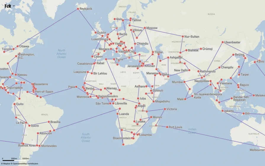
The “traveling salesman problem” is the problem in computer science of trying to calculate the route through a set of points that will visit them all with the smallest total distance traveled, and a traveling salesman traversal of our data points would give us pairs of points that are nearby neighbors. In 1982, John J. Bartholdi and Loren K. Platzman observed that ordering a set of points by their distances along a Hilbert space-filling-curve produced an approximation to the ideal route that was fast and easy to calculate and was good enough for their application (daily reallocation of Meals on Wheels delivery routes), and it is good enough for our purposes too.
I referred above to the average of those distances between pairs of points, but it turns out that in most geographic data sets, it is actually the logarithm of the distances that is normally distributed: that is, if the median distance between points is 4 miles, there will be equally many pairs that are 2 miles apart as 8 miles apart, rather than equally many that are 2 miles apart as 6 miles apart. This is because most things on the planet exist in clusters, with people clustered together in towns and cities, towns and cities clustered together in regions, and regions clustered together in continents.
So to calculate the representative distance between points in the data set, we take the geometric mean of the distances between pairs of (non-identical) points. That distance then translates into a zoom level. If the distance d is denominated in meters, the corresponding zoom level is ceil(log2(10000) - log2(d)), because the minimum distinguishable distance at zoom level 0 is approximately 10,000 meters (the circumference of the earth, divided by the 4096-unit size of the tile grid), and is cut in half with each increment to the zoom level.
This Hilbert ordering is also what allows me to refer above to “the area” that contains a cluster of buildings, and what enables the 40% of point features that are retained as you zoom out to be a spatially representative sample of the full data. Everything in Tippecanoe that is concerned with the density or locality or uniformity of feature locations is actually looking at features or pairs of features in Hilbert sequence rather than trying to do proper kernel density estimates. Tippecanoe accumulates the area of “polygon dust” buildings whose true shape is being lost in Hilbert sequence, and when it has accumulated enough area for something to be seen, it emits a placeholder at the location of the last “dust” building, confident that Hilbert locality makes that location suitably representative of the other lost features that have contributed area to it.
The distances within features
The zoom level calculation described above talks about point features, but we must also calculate an appropriate zoom level for polygon and line data. The first step of the process is still the same as with points features, but using a representative point for each polygon or line rather than the single point location that is inherent to a point feature. Tippecanoe formerly used the center of the bounding box of the feature as the representative point; now it uses one of the vertices of the feature, to avoid treating overlapping features as being extremely close together.
But if your data file is a set of country outlines, just being able to tell the countries apart from each other is not sufficient. You also need to be able to see the shape of each country, so we need to tile the features to a higher maximum zoom.
Fortunately the statistical properties that apply to representative points also basically apply to the distribution of vertices within any given feature and then to the distribution of representative distances across features. We take the geometric mean of the distances between vertices within each feature, and then take the geometric mean of those representative distances, and, if it indicates a higher zoom level than was calculated using the distances between features, use that higher zoom level as the maximum.
Case study: Wineries
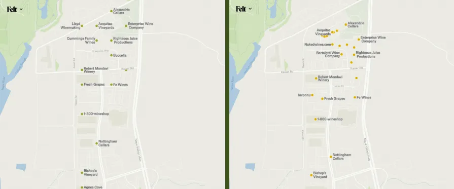
Problem solved, right? Well, not quite. One of the test data sets that we use frequently at Felt is a map of the wineries in the United States. For the most part, wine production is spatially distributed like anything else: with wineries clustered together in prime locations, which are part of regional clusters. But in this data set there are some clusters that are even more tightly clustered than usual, and if you uploaded this data and zoomed in on Napa, California, there were multiple wineries mapped at exactly the same locations, and the locations shown overall had an unpleasantly, unnaturally gridded shape to them.
Looking at several other data sets for comparison, I discovered that in focusing on the geometric mean distance between features, I had neglected to take into account that some data sets are much more tightly clustered than others. For those with relatively loose clustering, the geometric mean distance was choosing an appropriate maxzoom. But for those with tight clusters, it was choosing too low, so the clusters could be easily distinguished but not the individual points within those clusters.
I said above that the minimum distance between points is too small and too unrepresentative to be usable, and that is still true. But fortunately we can also calculate the standard deviation of the logs of the distances, not just their means, and use that to make a better decision.
Two standard deviations below the mean seemed like it should work well, because it should guarantee that 97.7% of feature pairs would have distinct locations. However, in practice, this number of additional zoom levels made processing excessively slow. We have backed off to 1.5 standard deviations below the mean, which should still guarantee that 93.3% of features can be distinguished, and is certainly plenty of for the tight cluster of wineries in Napa.
Case study: Rapid transit stations
However, it turns out that just being able to tell the features apart is not always enough. In particular, the station locations of Honolulu’s under-construction rapid transit system are generally a mile or so apart, so Tippecanoe would dutifully choose zoom level 5, with thousand-foot precision, as sufficient to make a map of them. But from the perspective of transit users, a thousand-foot error in the location of a station is enough to cause great confusion over where it actually is and how to find it. I resisted raising the zoom level, knowing that it would make other uploads much slower to process.
But fortunately we can still adjust other aspects of how Felt’s maps are created and displayed. In particular, we do not actually have to create our map tiles with a resolution of 4096x4096 tile units, and unlike some other map rendering software, Protomaps can support much higher resolutions. We now make adjustments in both directions: at the zoom levels below the maximum, we generate 1024x1024-unit tiles rather than 4096x4096, which look just as good at the resolution at which they are actually displayed, and are smaller to send over the network and faster to render. And for point data, at the maximum zoom level, we generate tiles with a resolution of up to 67108864x67108864, which gives a one-foot precision on the ground even at zoom level 1.
![]()
It would be nice if we could take more advantage of this very high resolution within the tiles to reduce the maximum zoom level while still retaining very high precision, speeding up processing. But one of the reasons we use multiple zoom levels is to reduce the ground area represented by each map tile, and therefore the number of features contained within it. A lower maximum zoom level would put too many features in each tile to load and render quickly. For the same reason, we still use 4096x4096 tiles at the maximum zoom level for line and polygon data, rather than also giving them extra precision, to avoid increasing the byte size of the tiles too much.