72% of total inflation occurred during just four periods.

A monthly dataset tracking the US Consumer Price Index from 1913 to present — decomposing 96.9% of cumulative purchasing power loss into four concentrated episodes that reshaped the American economy.
Eco3min Research · Last updated: · Frequency: Monthly · Coverage: Jan 1913 – Feb 2026
The US Consumer Price Index has tracked the cost of living since 1913, providing the longest continuous measure of inflation in the American economy. Over 113 years and 1,357 monthly observations, the CPI reveals a fundamental pattern that challenges the common perception of inflation as a slow, steady erosion: purchasing power destruction is not gradual. It arrives in concentrated bursts — episodic regime breaks separated by extended periods of relative stability. This page provides the complete monthly dataset with regime classification, episode tagging, and a decomposition analysis that quantifies exactly when and how the destruction occurred.
TL;DR
The US dollar has lost 96.9% of its purchasing power since 1914 — but this destruction was not gradual. Four inflationary episodes (WWI, WWII and the post-war boom, the Great Inflation of 1968–1982, and the post-COVID surge of 2021–2023) account for 72% of the total cumulative price increase, despite spanning only 29% of the total time. Inflation is not a slow leak. It is a series of regime breaks. Note: this dataset measures nominal purchasing power of a fixed dollar amount — it does not account for wage growth, productivity gains, or changes in living standards over the same period (see Methodology and Limitations).
Latest Observation — February 2026
327.5
CPI-U Index
2.4%
YoY Inflation
$3.05
Value of $100 (1914)
3.3%
Rolling 10Y Ann. Rate
Key Research Findings
- The US dollar has lost 96.9% of its purchasing power since January 1914. The CPI index has risen from 10.0 to 327.5 — a 32.7× multiplier — according to BLS data (series CPIAUCSL, retrieved March 2026). Equivalently, goods that cost $3.05 in 1914 would cost $100 today.
- This destruction was not gradual. Four concentrated inflationary episodes — WWI (1916–1920), WWII and the post-war boom (1941–1951), the Great Inflation (1968–1982), and the post-COVID surge (2021–2023) — account for 72% of the total cumulative price increase, despite spanning only 29% of the 113-year dataset.
- The Great Inflation of 1968–1982 alone accounts for 30.2% of all cumulative purchasing power destruction since 1914 — the single largest episode, exceeding either World War individually. During this 15-year period, the CPI rose from 34.1 to 97.7, nearly tripling the price level.
- Deflation — negative year-over-year CPI change — has occurred in 13.0% of all months since 1914 but has been entirely absent since April 2015. The longest sustained deflationary period was the Great Depression (1930–1933), when prices fell by approximately 26%.
- Of the 1,345 months with calculable year-over-year inflation, 61.6% exceeded the modern Federal Reserve’s 2% target. The median annual inflation rate across the full sample is 2.7% — above the current target. The current reading of 2.4% sits at the 46th percentile of the historical distribution.
- Important context: this dataset tracks nominal purchasing power only. Over the same 113-year period, real wages, productivity, and living standards rose substantially. The CPI measures the cost of a contemporaneous basket of goods — not the same basket — and does not capture quality improvements or entirely new categories of consumption. The 96.9% figure describes the erosion of a fixed dollar held as cash, not the erosion of household economic welfare. See Limitations for a full discussion.
1,357 monthly observations · CC BY 4.0 · Updated monthly · Methodology · Cite this dataset
1,357
Monthly Obs.
32.7×
CPI Multiplier
96.9%
Purchasing Power Lost
+23.7%
Highest YoY (Jun 1920)
−15.8%
Deepest Deflation (Jun 1921)
2.7%
Median YoY Inflation
Chart: US CPI Inflation Rate — Year-over-Year, Monthly (1914–2026)
US Consumer Price Index — Year-over-Year Change, Monthly, January 1914 to February 2026
CPI-U (BLS series CPIAUCSL, seasonally adjusted). Shaded areas: four major inflationary episodes accounting for 72% of cumulative purchasing power destruction.

Key Takeaway
The chart reveals that US inflation history is not a story of gradual erosion but of episodic shocks separated by extended periods of near-stability. The four shaded episodes dominate the visual — and the data confirms the visual: 72% of all cumulative price increases since 1914 occurred within these four windows. The current 2.4% reading represents a return to the historical median zone following the 2021–2023 post-COVID surge.
Sources: BLS (CPIAUCSL), Minneapolis Federal Reserve (historical CPI 1913–1946). Chart: Eco3min Research.
Updated monthly following BLS CPI release. Latest observation: February 2026.
How to Read This Chart
The chart plots the year-over-year percentage change in the Consumer Price Index (CPI-U) for every month from January 1914 to February 2026. Values above zero indicate inflation — the price level was higher than 12 months earlier. Values below zero indicate deflation — the price level was lower. The four shaded regions correspond to the major inflationary episodes identified in the dataset.
Several patterns emerge immediately. The pre-1945 era featured extreme volatility in both directions — including the 23.7% annual inflation of June 1920 and the −15.8% deflation of June 1921, a 39-point swing within a single year. From the mid-1950s onward, deflation essentially vanished from the US economy, and inflation became exclusively a positive phenomenon — occasionally surging, but never reversing into sustained price declines. For context on how interest rates responded to these inflation regimes, see our US Real Interest Rates dataset.
The post-2020 period is notable for producing the first sustained inflation above 5% since 1991 — briefly exceeded in July–August 2008 during the oil price spike, but not for consecutive months at this scale — and the first readings above 8% since January 1982. The subsequent normalization — from a peak of 9.0% in June 2022 to 2.4% by February 2026 — represents one of the fastest disinflation episodes in modern history, achieved without a recession. For a deeper examination of how the yield curve signaled the policy response, see our yield curve dataset.
Supplementary View: Purchasing Power on a Logarithmic Scale
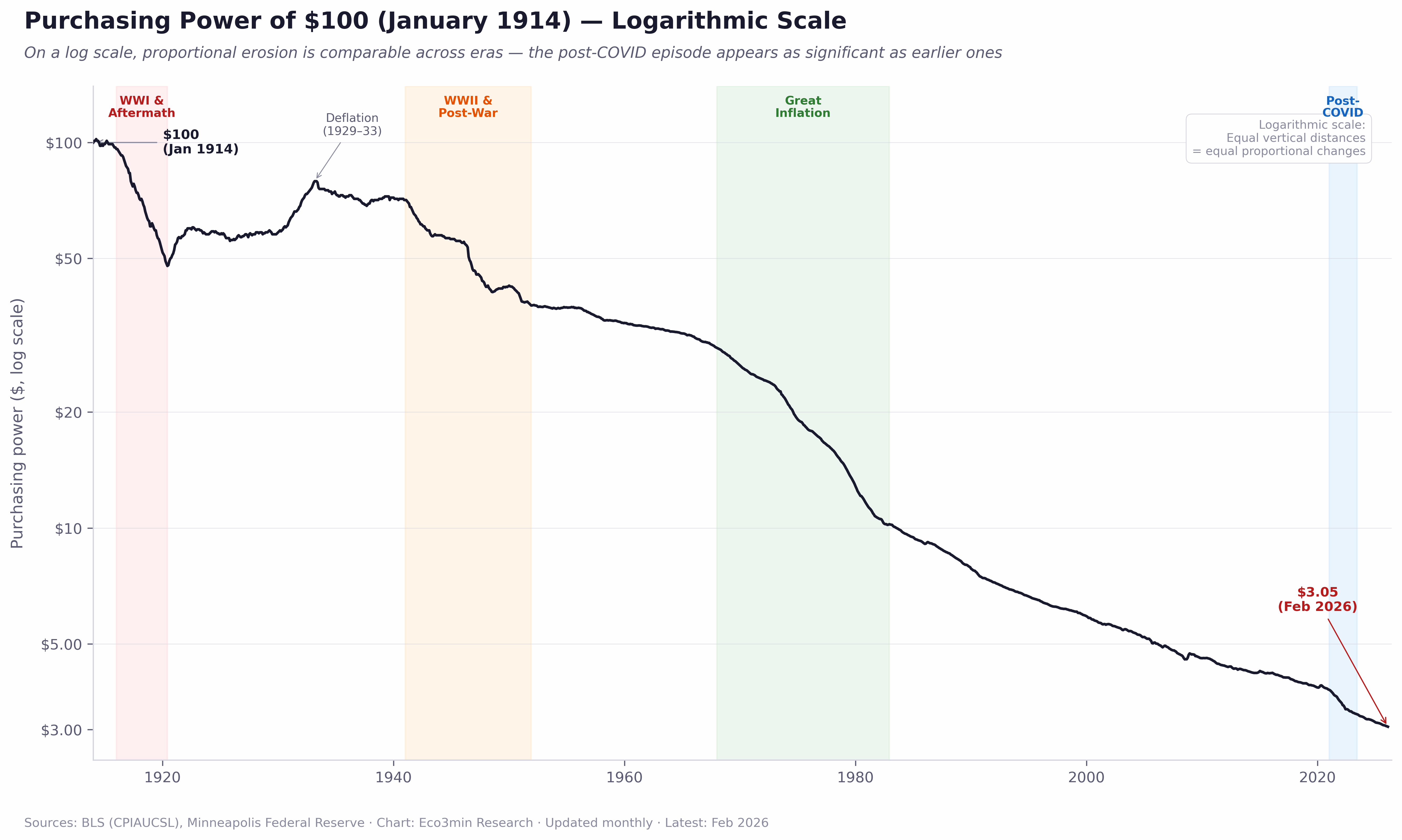
The hero chart at the top of this page uses a linear scale, which is intuitive but has a known limitation: it visually exaggerates early-period declines and compresses more recent ones. A 50% drop from $100 to $50 occupies the same vertical distance as a 50% drop from $10 to $5, even though the latter is proportionally identical. The logarithmic scale below corrects this by ensuring that equal proportional changes occupy equal vertical distances — making it possible to compare the severity of episodes across different base levels.
Purchasing Power of $100 (January 1914) — Logarithmic Scale
Same data as the linear chart above, plotted on a log scale. Equal vertical distances represent equal proportional changes. 1,357 monthly observations, January 1913 to February 2026.

What the Log Scale Reveals
On a log scale, the post-COVID episode — which appears minor on the linear chart — is clearly visible as a proportionally significant decline. The Great Depression deflation (the upward bump in the early 1930s) also becomes more prominent. The log view confirms that inflation episodes produce proportionally comparable damage regardless of the starting level, reinforcing the episode-decomposition analysis below. Both chart types are provided because they answer different questions: the linear chart shows how much remains; the log chart shows how fast it was lost.
Sources: BLS (CPIAUCSL), Minneapolis Federal Reserve (historical CPI). Chart: Eco3min Research.
Updated monthly. Latest observation: February 2026.
↓ PNG
↓ SVG
Free to reproduce with attribution. Cite this dataset
The Gradual Erosion Myth: Why the Standard Narrative Misleads
The dominant popular narrative about inflation operates on a simple metaphor: inflation is a slow, steady drip that quietly erodes purchasing power over time — like a faucet left running. This metaphor is intuitive, emotionally resonant, and empirically wrong.
The data tells a different story. Of the 1,345 months with calculable year-over-year inflation in this dataset, 342 — or 25.4% — recorded annual price changes between 0% and 2%. Another 430 months — 32.0% — recorded changes between 2% and 4%. Together, these “stable” and “moderate” periods represent 57.4% of all observations. In these months, the purchasing power erosion was indeed gradual: approximately 1–4 cents per dollar per year. If the entire 113-year period had proceeded at this pace, $100 in 1914 would still be worth approximately $12–20 today — a loss, certainly, but a manageable one.
Instead, $100 in 1914 is worth just $3.05 today — or equivalently, goods that cost $3.05 in 1914 would cost $100 today. The gap between the “gradual” scenario and reality is explained almost entirely by four concentrated episodes where annual inflation exceeded 5% for sustained periods. These episodes — driven by wartime mobilization, commodity shocks, monetary policy errors, and pandemic-era fiscal intervention — compressed decades of normal erosion into a few years each.
The mechanism is mathematical: inflation compounds. A single year of 10% inflation destroys as much purchasing power as five years of 2% inflation. When 10% inflation persists for three or four consecutive years — as it did during WWI, the post-war boom, and the Great Inflation — the compounding effect is devastating. This is why the distribution of destruction is so concentrated: 29% of the time produced 72% of the cumulative damage. For the interaction between these inflationary surges and equity market valuations, see our Real Rates vs CAPE dataset.
Important Analytical Context
Monetary regime changes. This dataset spans three fundamentally different monetary systems: the classical gold standard (pre-1914), the gold-exchange and Bretton Woods systems (1914–1971), and the post-Bretton Woods fiat currency regime (1971–present). Inflation behaved differently under each. Under the gold standard, deflation was a normal feature of the business cycle; under fiat currency with inflation targeting, it has been virtually eliminated. Comparing inflation rates across these regimes requires caution — a 5% reading under the gold standard reflected different structural forces than a 5% reading under modern central banking.
What this dataset does not measure. Purchasing power of a fixed dollar amount is not the same as household economic welfare. Over the same 113-year period, real median wages rose substantially, life expectancy nearly doubled, and entirely new categories of consumption — antibiotics, air travel, the internet — came into existence. A dollar buys less bread than in 1914, but the median worker earns far more dollars per hour, and those dollars buy goods and services that did not exist. This dataset isolates one dimension of the story — the nominal erosion of the monetary unit — and should not be interpreted as a comprehensive measure of economic decline.
Narrative Violation
The popular framing of inflation as gradual erosion obscures the empirical reality. 72% of all US purchasing power destruction since 1914 occurred during four inflationary episodes that together span only 29% of the total time. Inflation is not a slow leak. It is a series of regime breaks — each driven by a distinct macroeconomic mechanism, each concentrated in a window of a few years.
Episode Decomposition: Where the Destruction Happened
The four major inflationary episodes in the dataset can be decomposed by their contribution to the total cumulative log-CPI increase since January 1914. Using the natural logarithm of the CPI ratio ensures that each episode’s contribution is additive and comparable across different base levels. The total log increase from January 1914 (CPI 10.0) to February 2026 (CPI 327.5) is 3.49.
Contribution of Major Episodes to Cumulative Inflation
| Episode | Period | CPI Start → End | Price Increase | Share of Total |
|---|---|---|---|---|
| WWI & Aftermath | Jan 1916 – Jun 1920 | 10.4 → 20.9 | +101% | 20.0% |
| WWII & Post-War | Jan 1941 – Dec 1951 | 14.1 → 26.5 | +88% | 18.1% |
| Great Inflation | Jan 1968 – Dec 1982 | 34.1 → 97.7 | +187% | 30.2% |
| Post-COVID | Jan 2021 – Jun 2023 | 262.7 → 304.0 | +16% | 4.2% |
| All Other Periods | Remaining 80 years | — | — | 27.6% |
Episode Decomposition — Where 113 Years of Purchasing Power Destruction Actually Happened
Contribution of four major inflationary episodes to total cumulative CPI increase (log scale). 1,357 monthly observations, January 1913 to February 2026.

Key Takeaway
The Great Inflation of 1968–1982 — driven by the collapse of the Bretton Woods system, two oil shocks, and a decade of monetary policy errors — is the single largest contributor to cumulative price-level increase in the dataset, accounting for 30.2% of the total and exceeding either the WWI episode (20.0%) or the WWII episode (18.1%) individually. Together, the three wartime and post-war episodes account for 68.3% of all cumulative purchasing power erosion.
Sources: BLS (CPIAUCSL), Minneapolis Federal Reserve (historical CPI). Chart: Eco3min Research.
Updated monthly. Latest observation: February 2026.
Embed this chart in your article or newsletter:
Each Episode Had a Distinct Mechanism
The four episodes share a common outcome — rapid purchasing power destruction — but arose from fundamentally different macroeconomic mechanisms. Understanding these mechanisms is essential for distinguishing between inflationary environments rather than treating all inflation as identical.
WWI (1916–1920) · Wartime Demand Shock
Military mobilization, commodity shortages, and the gold standard’s inability to absorb fiscal expansion. Prices doubled in four years. The subsequent deflation of 1920–1921 (−15.8% YoY) was equally violent — the last major deflationary episode driven by peacetime adjustment.
WWII & Post-War (1941–1951) · Suppressed Then Released
Wartime price controls artificially suppressed inflation during 1943–1945. The removal of controls in 1946 released pent-up demand, producing a spike to 20.2% YoY in March 1947. The Korean War added a second pulse. Total price increase over the decade: 88%.
Great Inflation (1968–1982) · Policy Failure
The longest and most destructive episode. Triggered by the collapse of Bretton Woods, amplified by two oil shocks (1973, 1979), and sustained by a decade of accommodative monetary policy. CPI nearly tripled. Only the Volcker shock — federal funds rates exceeding 19% — ended it.
Post-COVID (2021–2023) · Fiscal-Supply Collision
Unprecedented fiscal stimulus collided with pandemic-disrupted supply chains. YoY CPI peaked at 9.0% in June 2022. The episode was resolved through aggressive Fed tightening without recession — the fastest disinflation in modern history.
Inflation by Decade: The Structural Shift from Volatility to Persistence
Aggregating the data by decade reveals a structural transformation in the behavior of US inflation. Before 1950, inflation was volatile in both directions — surging during wartime, collapsing during peacetime. The 1920s and 1930s both had median inflation below zero. After 1950, deflation essentially vanished, and inflation became a permanently positive phenomenon with varying intensity.
Median and Mean CPI Inflation by Decade
| Decade | Median YoY | Mean YoY | Max YoY | % Months > 5% | % Months < 0% |
|---|---|---|---|---|---|
| 1910s | 12.6% | 10.0% | 20.4% | 63.9% | 2.8% |
| 1920s | −0.6% | 0.1% | 23.7% | 9.2% | 53.3% |
| 1930s | −0.7% | −2.0% | 5.6% | 4.2% | 55.8% |
| 1940s | 3.5% | 5.7% | 20.2% | 45.0% | 8.3% |
| 1950s | 1.5% | 2.1% | 9.6% | 10.8% | 15.0% |
| 1960s | 1.6% | 2.3% | 5.9% | 8.3% | 0.0% |
| 1970s | 6.4% | 7.1% | 13.3% | 78.3% | 0.0% |
| 1980s | 4.3% | 5.6% | 14.6% | 30.8% | 0.0% |
| 1990s | 2.8% | 3.0% | 6.4% | 9.2% | 0.0% |
| 2000s | 2.8% | 2.6% | 5.5% | 1.7% | 8.3% |
| 2010s | 1.7% | 1.8% | 3.8% | 0.0% | 3.3% |
| 2020s | 3.1% | 3.9% | 9.0% | 28.8% | 0.0% |
Key Takeaway
The 1970s stand alone as the most inflationary decade in modern history: 78.3% of all months recorded year-over-year inflation above 5%, and the median annual rate was 6.4%. By contrast, the 2010s were the most stable decade since the 1950s — not a single month exceeded 3.8%. The 2020s, through their first six years, have already returned the US to an inflationary profile not seen since the 1980s.
The disappearance of deflation after 1955 is one of the most consequential structural changes in the dataset. Before the Federal Reserve adopted its modern inflation-targeting framework — and before the abandonment of the gold standard in 1971 — deflationary adjustments were a normal feature of the business cycle. Prices went up during booms and came back down during busts. The post-Bretton Woods monetary system has effectively eliminated the “down” part of this cycle, replacing it with an asymmetry: inflation varies between “low” and “high,” but prices only go up. For a detailed analysis of how Federal Reserve policy decisions contributed to this structural shift, see our Fed Funds Rate study.
The Inflation-Targeting Era (Post-1995)
The data also tells a story that the headline figures can obscure: inflation targeting works. Since the Federal Reserve informally adopted a 2% inflation target in the mid-1990s, the median year-over-year CPI reading has been 2.4% and the mean 2.5% — remarkably close to target. The post-COVID surge (2021–2023) represents the only significant excursion above 5% in this 30-year period, and it was resolved in under three years without a recession. Of the total 96.9% purchasing power loss since 1914, only approximately 21% occurred during the post-1995 inflation-targeting era, despite this period representing roughly 25% of the total time span. This suggests that the modern monetary policy framework, while imperfect, has substantially reduced the frequency and severity of inflationary episodes compared to earlier regimes.
Inflation Regime Classification: Seven States of the Price Level
The dataset classifies every monthly observation into one of seven inflation regimes based on the year-over-year CPI change. This classification enables researchers to filter the data by macroeconomic environment and study how asset returns, policy decisions, and consumer behavior differ across inflationary regimes.
Regime Distribution — 1,345 Monthly Observations with YoY Data
| Regime | YoY Range | Months | Share | Dominant Periods |
|---|---|---|---|---|
| Crisis | Above +10% | 118 | 8.8% | WWI, WWII aftermath, 1979–1981 |
| High | +6% to +10% | 125 | 9.3% | 1973–1982, 2022 |
| Elevated | +4% to +6% | 155 | 11.5% | 1968–1972, 1988–1991, 2021 |
| Moderate | +2% to +4% | 430 | 32.0% | 1990s–2020s baseline |
| Stability | 0% to +2% | 342 | 25.4% | 1920s, 1950s–1960s, 2010s |
| Mild Deflation | 0% to −2% | 88 | 6.5% | 1920s, 1930–1932, 2009 |
| Deflation | Below −2% | 87 | 6.5% | 1921, 1930–1933, 1938 |
- The “Moderate” regime (2–4% YoY) is the most common single state, representing 32.0% of all observations — suggesting that mild inflation above the current 2% target has historically been the normal condition, not the exception.
- “Crisis” inflation (above 10%) has occurred in 8.8% of months — nearly one in eleven. Every instance was associated with a specific identifiable shock: wartime mobilization, the removal of price controls, or an oil price surge.
- Deflation in all forms (Mild + Deep) represents 13.0% of observations, but nearly 90% of these months occurred before 1955. The last sustained deflation was in 2009 (trough of −2.0% YoY in July), driven by the Global Financial Crisis.
- The current reading of 2.4% places February 2026 squarely in the “Moderate” regime — at the lower end of its range and near the long-run median of 2.7%.
Interactive Tool
Inflation Impact Calculator
Select a starting year and amount to see how inflation has eroded purchasing power. Based on 1,357 monthly CPI observations (1913–2026).
1970
19142025
$1,000
$100$100,000
—
Value in Feb 2026
—
Purchasing Power Lost
—
CPI Multiplier
—
Annualized Inflation
Select a year to see results.
Historical Turning Points: Five Moments That Reshaped the Price Level
June 1920 — The All-Time Inflation Peak
Year-over-year CPI inflation reached 23.7% in June 1920, the highest reading in the 113-year dataset. The CPI had risen from 10.4 in January 1916 to 20.9 by June 1920 — a doubling in just over four years, driven by wartime demand, commodity shortages, and the inability of the gold standard to absorb the fiscal expansion required by WWI. The subsequent reversal was equally dramatic: by June 1921, CPI YoY had plunged to −15.8%, producing the most violent deflationary adjustment in modern American history. Together, the 1920–1921 episode is the only instance in the dataset where double-digit inflation was followed by double-digit deflation within a single year.
March 1933 — The Deflationary Trough
The CPI reached 12.6 in March 1933, down from 17.1 in January 1930 — a cumulative decline of 26.3% over three years. This deflation was not the benign variety associated with productivity gains; it reflected a catastrophic collapse in demand, mass unemployment, and a banking crisis that destroyed credit. The purchasing power of a dollar rose sharply during this period — but it was a Pyrrhic gain, as the income available to spend those more-powerful dollars was collapsing even faster. The experience of the Great Depression permanently altered the US policy establishment’s tolerance for deflation, ultimately contributing to the modern monetary framework’s asymmetric bias toward accepting mild inflation over any deflation.
March 1980 — The Volcker Peak
CPI YoY reached 14.6% in March 1980 — the highest reading since 1947. The CPI index stood at 80.1, up from 34.1 at the start of 1968. The Great Inflation had persisted for over a decade, driven by a cascading series of policy errors, supply shocks, and structural changes. Fed Chair Paul Volcker’s decision to target monetary aggregates rather than interest rates — pushing the federal funds rate above 19% — produced the most severe monetary tightening in post-war history. The resulting recession broke the inflationary psychology, but at the cost of 10.8% unemployment. For context on how real interest rates responded, real rates exceeded +9% in 1982–1984.
June 2022 — The Post-COVID Peak
CPI YoY reached 9.0% in June 2022, the highest since January 1982 — driven by the collision of pandemic-era fiscal stimulus (approximately $5.2 trillion in federal spending between March 2020 and March 2021) with disrupted global supply chains. The CPI rose from 262.7 in January 2021 to 296.3 by September 2022. Unlike previous episodes, the subsequent disinflation was achieved without a recession: CPI YoY fell from 9.0% to 3.0% in less than 18 months, aided by supply chain normalization and the Federal Reserve’s fastest tightening cycle in four decades. For how credit spreads responded to this period, see our credit dataset.
February 2026 — Current Observation
The CPI stands at 327.5, with year-over-year inflation of 2.4% — at the 46th percentile of the full historical distribution. The rolling 10-year annualized inflation rate is 3.3%, above the Federal Reserve’s 2% target but at the 113-year mean. The current environment reflects a post-surge normalization, with inflation decelerating from the 2021–2023 episode but not yet returning to the sub-2% readings that characterized the 2010s. The key question for 2026 is whether the structural factors that kept inflation below 2% for the decade prior to COVID — globalization, technology-driven productivity gains, and demographic trends — will reassert themselves, or whether the post-pandemic economy has shifted to a permanently higher baseline.
Methodology
This dataset combines two official data sources — the BLS historical CPI tables (1913–1946) and the FRED CPIAUCSL series (1947–present) — into a single monthly panel covering 113 years. All derived variables are computed from the CPI index level.
Consumer Price Index. The CPI-U (Consumer Price Index for All Urban Consumers) measures the average change in prices paid by urban consumers for a basket of goods and services. The base period is 1982–84 = 100. Data from 1913 to 1946 is sourced from the BLS supplemental historical tables; data from 1947 onward is sourced from FRED series CPIAUCSL (seasonally adjusted). For a discussion of the differences between CPI and PCE inflation measures, see our PCE Inflation dataset.
Year-over-year inflation. Computed as the percentage change in the CPI index level from 12 months prior. This is a date-based calculation (not row-based), ensuring accuracy even when individual months are missing from the source data.
Purchasing power index. The value of $100 in January 1914 purchasing power, computed as (CPIJan 1914 / CPIt) × 100 for each month t.
Episode share calculation. Each episode’s contribution to total cumulative inflation is computed using the natural logarithm of the CPI ratio: ln(CPIend / CPIstart) / ln(CPIFeb 2026 / CPIJan 1914). This ensures additivity across episodes.
CPI YoYt = (CPIt / CPIt−12 − 1) × 100 | PPt = (CPIJan 1914 / CPIt) × 100
Episode Selection Criteria
The four inflationary episodes were identified using a combination of quantitative thresholds and historical periodization. An episode is defined as a period meeting at least one of the following criteria: (1) year-over-year CPI exceeds 5% for 12 or more consecutive months, or (2) the cumulative log-CPI increase over the episode exceeds 0.15 (approximately a 16% price-level increase). Episode boundaries are extended to include the full acceleration and deceleration phases — from the month when YoY inflation first crosses 3% on the way up to the month when it falls back below 3% on the way down — to capture the complete inflationary cycle rather than just the peak.
This selection identifies the same four episodes that are conventionally recognized in the macroeconomic history literature (Reis, 2021; Summers, 2022). The “All Other Periods” residual (27.6% of cumulative inflation) represents the baseline erosion from moderate inflation during the remaining 80 years — a meaningful contribution that reinforces the point that even “quiet” inflation compounds over time.
Dataset Design
| Variable | Description | Unit | Source |
|---|---|---|---|
| date | Monthly observation date | YYYY-MM | — |
| cpi_index | CPI-U, seasonally adjusted | Index (1982-84=100) | BLS / FRED |
| cpi_yoy_pct | Year-over-year CPI change | Percent | Calculated |
| cpi_mom_pct | Month-over-month CPI change | Percent | Calculated |
| purchasing_power_100 | Value of $100 (Jan 1914 base) | Dollars | Calculated |
| pct_loss_since_1914 | Cumulative loss since Jan 1914 | Percent | Calculated |
| inflation_regime | Seven-state classification | Categorical | Eco3min |
| episode | Major episode tag | Categorical | Eco3min |
| rolling_10y_ann_inflation | 10-year annualized inflation | Percent | Calculated |
| decade | Decade classification | Integer | Calculated |
Python Reproduction Code
import pandas as pd
import numpy as np

# Load CPIAUCSL from FRED (1947–present)
df_fred = pd.read_csv(
    "https://fred.stlouisfed.org/graph/fredgraph.csv?id=CPIAUCSL"
)
df_fred.columns = ['date', 'cpi_index']

# For 1913–1946: use BLS historical supplemental tables
# Available at bls.gov/cpi/tables/supplemental-files/

# Compute YoY inflation (date-based, not row-based)
df['date'] = pd.to_datetime(df['date'])
df = df.set_index('date')
df['cpi_yoy_pct'] = df['cpi_index'].pct_change(12) * 100

# Purchasing power of $100 (Jan 1914 base)
cpi_1914 = df.loc['1914-01', 'cpi_index']
df['purchasing_power'] = (cpi_1914 / df['cpi_index']) * 100

# Episode share: log decomposition
total_log = np.log(df['cpi_index'].iloc[-1] / cpi_1914)
ep_log = np.log(cpi_end / cpi_start)
share = ep_log / total_log * 100

# Export
df.to_csv("us-cpi-inflation-history-1913-present.csv")
Explore more macroeconomic datasets:
Eco3min Macro Data Hub
— inflation, yield curves, equity returns, credit spreads and global indicators.
Dataset Download & Reproducibility
The complete dataset is provided in open formats for quantitative analysis and academic research. Updated monthly following the BLS CPI release.
License: Creative Commons Attribution 4.0 (CC BY 4.0). Free for research, academic, and journalistic use with attribution to Eco3min.
For researchers: The dataset includes episode tags, regime classifications, and rolling metrics that enable direct use in regime-switching models, inflation-forecasting frameworks, and asset-class return analysis by inflation environment. All variables required to replicate the episode decomposition and regime classification are included in the CSV/XLSX download.
Data Sources & References
- Primary
U.S. Bureau of Labor Statistics (BLS) — Consumer Price Index for All Urban Consumers (CPI-U), series CPIAUCSL. Seasonally adjusted, monthly, 1947–present. - Primary
BLS Supplemental Historical Tables — Historical CPI-U monthly data, 1913–1946 (1982-84=100 base). - Primary
Federal Reserve Bank of St. Louis (FRED) — CPIAUCSL series, programmatic access and retrieval. - Primary
Federal Reserve Bank of Minneapolis — Consumer Price Index, 1913–present. Historical series compilation and inflation calculator. - Research
Reis (2021) — “Losing the Inflation Anchor,” Brookings Papers on Economic Activity. Analysis of inflation expectations de-anchoring risk. - Research
Summers (2022) — “Comparing Past and Present Inflation,” NBER Working Paper. Methodology for adjusting historical CPI for composition changes. - Reference
National Bureau of Economic Research (NBER) — US Business Cycle Dates for recession shading reference.
Methodological Limitations
- Nominal purchasing power only — no wage or income context. This dataset measures the erosion of a fixed dollar amount held as cash. It does not account for wage growth, investment returns, or productivity gains. Over the same 113-year period, real (inflation-adjusted) median wages rose substantially. The 96.9% purchasing power loss describes what happened to a dollar stored under a mattress — not to a dollar earned, invested, or spent. Any interpretation of this dataset as a measure of household welfare decline is a misreading of what the CPI measures.
- CPI basket composition changes. The basket of goods and services tracked by the CPI has changed substantially since 1913. Categories like “horse feed” have been removed; categories like “smartphones” have been added. This means the CPI does not measure the same thing across its full history — it measures the cost of a contemporaneous lifestyle, not a fixed one.
- Quality adjustment (hedonic pricing). Since 1998, the BLS has applied hedonic quality adjustments to some CPI components. This methodology lowers measured inflation when product quality improves (e.g., a computer that is twice as fast at the same price counts as a price decline). Critics argue this understates experienced inflation; the BLS argues it produces a more accurate cost-of-living measure.
- Substitution bias. The CPI-U uses a Laspeyres-type index that does not fully account for consumer substitution when relative prices change. The Chained CPI (C-CPI-U) addresses this but is only available from December 1999.
- Shelter measurement. The CPI uses “owners’ equivalent rent” to measure housing costs for homeowners, which may not reflect actual mortgage payment experiences. This component represents approximately 26% of the current CPI basket and is measured with a substantial lag.
- Three monetary regimes, one dataset. This dataset spans the classical gold standard (pre-1914), the gold-exchange and Bretton Woods systems (1914–1971), and the post-Bretton Woods fiat currency regime (1971–present). Inflation behavior differs structurally across these regimes — deflation was normal under the gold standard and has been virtually eliminated under fiat currency. Cross-regime comparisons should be made with this context in mind.
- Pre-1947 data quality. Monthly CPI data before 1947 was not collected with the same geographic coverage, sample size, or methodological rigor as modern data. The BLS considers the series comparable but notes that early estimates should be treated with appropriate caution.
- Seasonally adjusted vs. not seasonally adjusted. This dataset uses the seasonally adjusted series (CPIAUCSL) from 1947 onward. Pre-1947 data is not seasonally adjusted, as BLS seasonal factors are not available for the historical series. Year-over-year comparisons minimize the impact of this inconsistency.
Frequently Asked Questions
How much has the US dollar lost in purchasing power since 1914?
As of February 2026, the US dollar has lost 96.9% of its purchasing power relative to January 1914. This means that $100 in 1914 would buy only approximately $3.05 worth of goods today — or equivalently, goods that cost $3.05 in 1914 would cost $100 today. The CPI has risen from 10.0 in January 1914 to 327.5 in February 2026 — a 32.7× multiplier. However, this erosion was not gradual: four concentrated inflationary episodes account for 72% of the total cumulative price increase.
What was the highest inflation rate in US history?
The highest year-over-year CPI inflation rate in the dataset is 23.7%, recorded in June 1920 during the post-World War I commodity boom. In the post-WWII era, the highest readings were 20.2% in March 1947 (following the removal of wartime price controls) and 14.6% in March 1980 (during the second oil shock). The post-COVID peak was 9.0% in June 2022 — the highest since January 1982.
When was the last time the US experienced deflation?
The last month with negative year-over-year CPI change was April 2015, when YoY inflation briefly dipped below zero due to the collapse in oil prices. The last sustained deflationary episode was during the Global Financial Crisis: from January through October 2009 (with a marginal positive reading of +0.01% in February), CPI YoY was negative, reaching a trough of −2.0% in July 2009. Before that, sustained deflation had not occurred since the Great Depression of the 1930s.
What is the average inflation rate over the past 100 years?
Over the full 1914–2026 sample, the mean year-over-year CPI inflation rate is 3.3% and the median is 2.7%. However, this average masks extreme variation: the 1970s had a median of 6.4%, while the 2010s had a median of just 1.7%. The rolling 10-year annualized inflation rate as of February 2026 is 3.3%, which is at the long-run mean.
Is current US inflation high by historical standards?
As of February 2026, US CPI inflation of 2.4% year-over-year is at the 46th percentile of the historical distribution — essentially at the median. It is above the Federal Reserve’s 2% target but below the 113-year mean of 3.3%. The post-COVID surge (9.0% peak in June 2022) has largely normalized, and the current reading is consistent with the “Moderate” inflation regime (2–4% YoY) that has been the most common state in the dataset.
Can I use this dataset for academic research?
Yes. The complete dataset is available in CSV and Excel formats under a Creative Commons Attribution 4.0 (CC BY 4.0) license. It includes the CPI index, year-over-year and month-over-month changes, purchasing power calculations, inflation regime classifications, episode tags, and rolling 10-year metrics. Please cite as: Eco3min Research (2026), “US CPI Inflation History Dataset (1913–Present).”
Source
Eco3min Research (2026)
US CPI Inflation History — Consumer Price Index Dataset (1913–Present).
Eco3min Macro Data Hub — Research Indicators.
Eco3min.fr/en/us-inflation-is-not-linear/
Dataset released under the Creative Commons Attribution 4.0 International License (CC BY 4.0).
Free to reuse with attribution.
This article provides economic and financial analysis for informational purposes only. It does not constitute investment advice or a personalized recommendation. Any investment decision remains the sole responsibility of the reader.