In Part 1, I described how duplicating a block of seven middle layers in Qwen2-72B — no weight changes, no training — produced the #1 model on the HuggingFace Open LLM Leaderboard. The method, which I called RYS (Repeat Your Self), was discovered using nothing but hard math probes and EQ-Bench on a pair of RTX 4090s.
That was mid-2024. Since then, a flood of strong open-source models has arrived — Qwen3.5, MiniMax, GLM-4.7, and others — and I finally have enough compute at home to scan them properly.
So the question driving this post is simple: was RYS a fluke of Qwen2-72B, or is it a general property of Transformers?
More specifically:
- Does relayering still help on stronger modern models?
- Which modifications actually earn their extra layers?
- If two good motifs help independently, do they stack?
The short answer is yes, relayering survives. The longer answer took 3,024 beam search candidates, a surrogate model scoring 2 million configurations, and a unified validation sweep to work out properly. Along the way, I also released the scanning code and a set of new RYS models.
Let’s get into it!
Why Qwen3.5-27B
The Qwen3.5 family dropped around Chinese New Year 2026 and immediately became the darling of the LocalLLaMA crowd. Strong benchmarks, good vibes, well-engineered.
I’m most interested in models over 200B — that’s what my dual Grace-Hopper system is built for — but the broader community runs smaller models, and the 27B size hits a sweet spot: large enough to have interesting internal structure, small enough that most people with a decent GPU can actually use a RYS variant.
There’s also a scientific reason. In Part 1, I noted that smaller models tend to have more entangled functional anatomy — encoding, reasoning, and decoding are less cleanly separated. If RYS still works on a 27B model, that tells us the circuit structure is robust even when the brain is more compact. If it doesn’t work, that’s also interesting.
(MiniMax M2.5 and others are in the pipeline. The Hopper is grinding. More heatmaps to come.)
Seeing the Anatomy Directly
Before we get to the optimisation work, I want to show something new. In Part 1, the three-phase hypothesis — early layers encode, middle layers reason, late layers decode — was inferred indirectly from the Base64 observation and the heatmap patterns. It was a good story, but I couldn’t see the anatomy directly. I could only see its consequences.
That changed thanks to Evan Maunder, who ran a beautifully simple experiment after reading Part 1. He fed three semantically identical sentences through a model — one in English, one in Mandarin, one encoded as Base64 — and measured the cosine similarity of their hidden states at every layer. The results showed exactly the three-phase structure: rapid convergence in the first few layers (encoding), near-perfect similarity through the middle (reasoning in a format-agnostic space), and divergence in the final layers (decoding back to surface form).
I wanted to push this further. Evan’s experiment compared languages while holding content fixed. But what happens when you vary both? If the middle layers really operate in a universal “thinking space,” then two sentences about the same topic should be more similar than two sentences in the same language about different topics — even if one is in English and the other is in Chinese.
Using language samples from:
- EN = English
- ZH = Chinese
- AR = Arabic
- RU = Russian
- JA = Japanese
- KO = Korean
- HI = Hindi
- FR = French
And on the following topics:
- SCIENCE
- POEM
- HISTORY
- COOKING
- LAW
- MEDICAL
- SPORTS
- ECONOMY
Full Dataset (Click to expand)
- "EN_SCIENCE": "Photosynthesis converts light energy into chemical energy stored in glucose."
- "ZH_SCIENCE": "光合作用把光能转化为储存在葡萄糖中的化学能。"
- "AR_SCIENCE": "تحول عملية التمثيل الضوئي طاقة الضوء إلى طاقة كيميائية مخزنة في الجلوكوز."
- "RU_SCIENCE": "Фотосинтез преобразует световую энергию в химическую энергию, запасенную в глюкозе."
- "JA_SCIENCE": "光合成は光エネルギーをグルコースに蓄えられる化学エネルギーへ変換する。"
- "KO_SCIENCE": "광합성은 빛 에너지를 포도당에 저장되는 화학 에너지로 바꾼다."
- "HI_SCIENCE": "प्रकाश संश्लेषण प्रकाश ऊर्जा को ग्लूकोज़ में संचित रासायनिक ऊर्जा में बदलता है।"
- "FR_SCIENCE": "La photosynthese transforme l'energie lumineuse en energie chimique stockee dans le glucose."
- "EN_POEM": "At dusk, the moon lays silver on the tide while the wind carries a quiet song."
- "ZH_POEM": "黄昏时,月亮把银辉铺在潮汐上,风里带着一首安静的歌。"
- "AR_POEM": "عند الغسق يفرش القمر فضته على المد وتحمل الريح اغنية هادئة."
- "RU_POEM": "В сумерках луна расстилает серебро по приливу, а ветер несет тихую песню."
- "JA_POEM": "夕暮れに月は潮の上へ銀を敷き、風は静かな歌を運ぶ。"
- "KO_POEM": "해질 무렵 달빛이 밀물 위에 은빛을 깔고 바람은 조용한 노래를 실어 나른다."
- "HI_POEM": "सांझ में चांद ज्वार पर चांदी बिछा देता है और हवा एक शांत गीत लेकर चलती है।"
- "FR_POEM": "Au crepuscule, la lune pose de l'argent sur la maree tandis que le vent porte une chanson tranquille."
- "EN_HISTORY": "The printing press accelerated the spread of knowledge across Europe in the fifteenth century."
- "ZH_HISTORY": "印刷机在十五世纪加速了知识在欧洲的传播。"
- "AR_HISTORY": "سرعت المطبعة انتشار المعرفة عبر اوروبا في القرن الخامس عشر."
- "RU_HISTORY": "Печатный станок ускорил распространение знаний по Европе в пятнадцатом веке."
- "JA_HISTORY": "活版印刷は十五世紀のヨーロッパで知識の拡散を加速させた。"
- "KO_HISTORY": "인쇄기는 15세기 유럽 전역으로 지식이 퍼지는 속도를 높였다."
- "HI_HISTORY": "मुद्रण यंत्र ने पंद्रहवीं शताब्दी में पूरे यूरोप में ज्ञान के प्रसार को तेज कर दिया।"
- "FR_HISTORY": "L'imprimerie a accelere la diffusion du savoir en Europe au quinzieme siecle."
- "EN_COOKING": "To make soup, simmer onions, carrots, and beans until the broth becomes rich and fragrant."
- "ZH_COOKING": "做汤时,把洋葱、胡萝卜和豆子慢炖,直到汤汁变得浓郁而香。"
- "AR_COOKING": "لتحضير الحساء، اطه البصل والجزر والفاصوليا على نار هادئة حتى يصبح المرق غنيا وعطرا."
- "RU_COOKING": "Чтобы приготовить суп, томите лук, морковь и фасоль, пока бульон не станет насыщенным и ароматным."
- "JA_COOKING": "スープを作るには、玉ねぎ、にんじん、豆を煮込み、だしが濃く香るまで待つ。"
- "KO_COOKING": "수프를 만들려면 양파와 당근, 콩을 천천히 끓여 국물이 진하고 향긋해질 때까지 익힌다."
- "HI_COOKING": "सूप बनाने के लिए प्याज, गाजर और बीन्स को धीमी आंच पर पकाएं, जब तक शोरबा गाढ़ा और सुगंधित न हो जाए।"
- "FR_COOKING": "Pour preparer une soupe, faites mijoter des oignons, des carottes et des haricots jusqu'a ce que le bouillon devienne riche et parfume."
- "EN_LAW": "A contract becomes enforceable when both parties agree to clear terms and exchange consideration."
- "ZH_LAW": "当双方同意明确条款并交换对价时,合同就具有可执行性。"
- "AR_LAW": "يصبح العقد قابلا للتنفيذ عندما يوافق الطرفان على شروط واضحة ويتبادلان المقابل."
- "RU_LAW": "Договор становится подлежащим исполнению, когда обе стороны согласны с ясными условиями и обмениваются встречным
- предоставлением."
- "JA_LAW": "契約は、当事者双方が明確な条件に合意し、対価を交わしたときに執行可能になる。"
- "KO_LAW": "계약은 양측이 명확한 조건에 동의하고 대가를 교환할 때 집행 가능해진다."
- "HI_LAW": "जब दोनों पक्ष स्पष्ट शर्तों पर सहमत होते हैं और प्रतिफल का आदान-प्रदान करते हैं, तब अनुबंध लागू करने योग्य बनता है।" "FR_LAW": "Un contrat devient executoire lorsque les deux parties acceptent des conditions claires et echangent une contrepartie."
- "EN_MEDICAL": "Vaccination trains the immune system to recognize a pathogen before a real infection occurs."
- "ZH_MEDICAL": "疫苗接种会训练免疫系统在真正感染发生前识别病原体。"
- "AR_MEDICAL": "يدرب التطعيم الجهاز المناعي على التعرف على الممرض قبل حدوث عدوى حقيقية."
- "RU_MEDICAL": "Вакцинация обучает иммунную систему распознавать патоген до того, как произойдет настоящая инфекция."
- "JA_MEDICAL": "ワクチン接種は、実際の感染が起こる前に免疫系が病原体を見分けられるようにする。"
- "KO_MEDICAL": "백신 접종은 실제 감염이 일어나기 전에 면역 체계가 병원체를 알아보도록 훈련한다."
- "HI_MEDICAL": "टीकाकरण प्रतिरक्षा तंत्र को वास्तविक संक्रमण से पहले रोगजनक को पहचानना सिखाता है।"
- "FR_MEDICAL": "La vaccination entraine le systeme immunitaire a reconnaitre un agent pathogene avant qu'une veritable infection ne se produise."
- "EN_SPORTS": "A relay team wins when each runner exchanges the baton cleanly and maintains speed through every leg."
- "ZH_SPORTS": "接力队在每位跑者顺利交接接力棒并在每一棒保持速度时才能获胜。"
- "AR_SPORTS": "يفوز فريق التتابع عندما يسلم كل عداء العصا بسلاسة ويحافظ على السرعة في كل مرحلة."
- "RU_SPORTS": "Эстафетная команда побеждает, когда каждый бегун чисто передает палочку и сохраняет скорость на каждом этапе."
- "JA_SPORTS": "リレーチームは、各走者がバトンを確実に渡し、すべての区間で速度を保つと勝てる。"
- "KO_SPORTS": "계주 팀은 각 주자가 배턴을 깔끔하게 넘기고 모든 구간에서 속도를 유지할 때 승리한다."
- "HI_SPORTS": "रिले टीम तब जीतती है जब हर धावक बैटन को साफ़ी से सौंपता है और हर चरण में गति बनाए रखता है।"
- "FR_SPORTS": "Une equipe de relais gagne lorsque chaque coureur transmet le temoin proprement et conserve sa vitesse sur chaque portion."
- "EN_ECONOMY": "When interest rates rise, borrowing often slows and household spending can weaken."
- "ZH_ECONOMY": "当利率上升时,借贷往往会放缓,家庭支出也可能减弱。"
- "AR_ECONOMY": "عندما ترتفع اسعار الفائدة، يتباطا الاقتراض غالبا وقد يضعف انفاق الاسر."
- "RU_ECONOMY": "Когда процентные ставки растут, заимствования часто замедляются, а расходы домохозяйств могут ослабеть."
- "JA_ECONOMY": "金利が上がると、借り入れは鈍り、家計支出も弱くなりやすい。"
- "KO_ECONOMY": "금리가 오르면 차입이 둔화되고 가계 지출도 약해질 수 있다."
- "HI_ECONOMY": "जब ब्याज दरें बढ़ती हैं, तो उधार लेना अक्सर धीमा पड़ जाता है और घरेलू खर्च कमजोर हो सकता है।"
- "FR_ECONOMY": "Lorsque les taux d'interet augmentent, l'emprunt ralentit souvent et les depenses des menages peuvent faiblir."
Pairwise, that is $C(64, 2) = 2016$ natural-language comparisons. Then I computed pairwise cosine similarity of the pooled hidden states at every layer. This gives us 3 categories:
- 224 Cross-language, Same content: comparisons (in red)
- 224 Same language, Different content: comparisons (in green)
- 1568 Cross-language, Different content: comparisons (in blue)
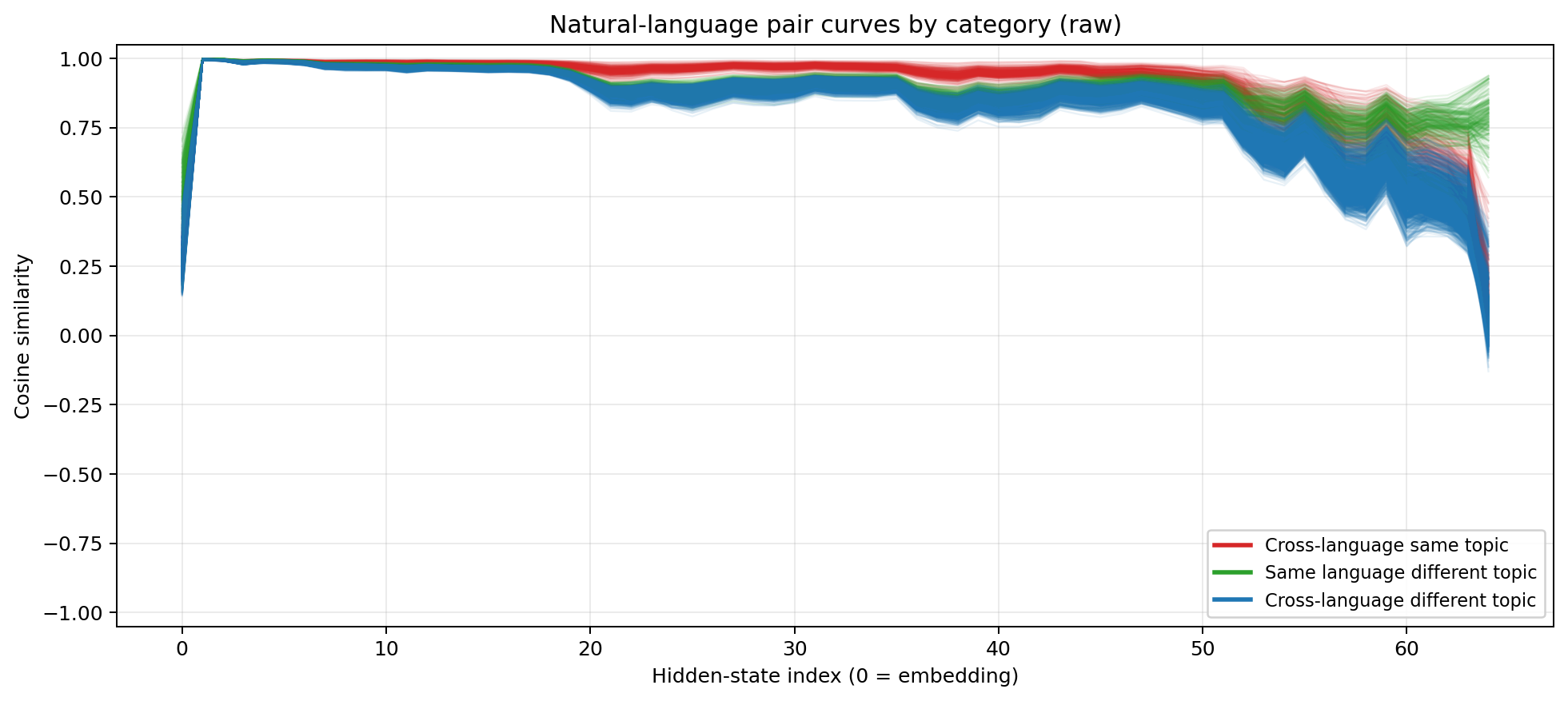
Raw cosine similarity across layers. All pairs converge rapidly in the first few layers. The interesting divergence happens in the mid-to-late stack.
The raw plot already tells a story. All pairs start at moderate similarity (0.2–0.6 at the embedding layer), then rapidly converge to near-1.0 by about layer 3. Through the mid-stack, they stay high but begin to separate. The red line (Cross-language, Same content:) stays above the green line (Same language, Different content:), which itself stays above the blue lines (Cross-language, Different content:), from roughly layer 15 onward. The model’s internal representation cares more about what you’re saying than what language you’re saying it in.
The aggregate numbers:
- Cross-language, same content: 0.902 mean similarity
- Same-language, different content: 0.891 mean similarity
- Cross-language, different content: 0.829 mean similarity
But the raw cosine similarities are dominated by a large shared component — every hidden state at a given layer lives in roughly the same region of the space (the “hyper-cone” effect that’s well-documented in the literature). To see the structure more clearly, I applied per-layer centering: subtract the mean vector across all four inputs at each layer, then re-normalise before computing cosine similarity. This strips out the “I’m at layer N” component and reveals only how the representations differ from each other.
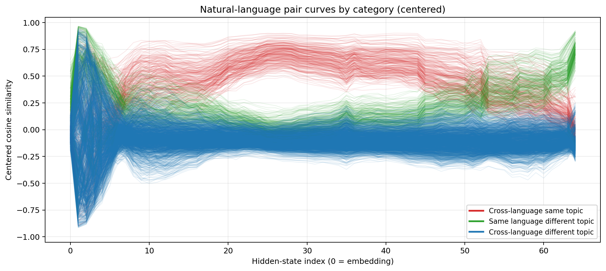
Centered cosine similarity. After removing the shared component, the organisation becomes stark.
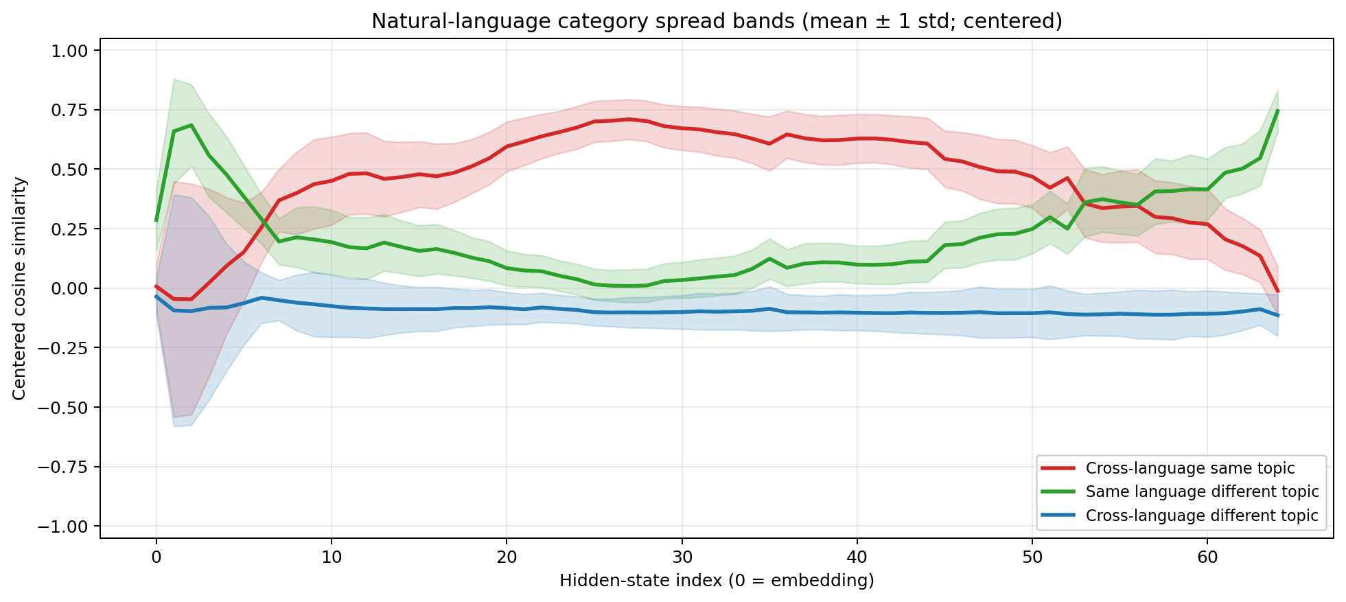
Centered cosine similarity. Mean/STD spread-band plots
Now the anatomy is unmistakable. Three phases:
Encoding (layers 0–5). Wild oscillation. The model is doing heavy lifting to normalise radically different surface forms. The model knows it’s reading English or Chinese, and the representations reflect that.
Reasoning (layers ~10–45). The red line dominates. These are the cross-language same-content pairs. The model has converged on a representation where content identity matters far more than language identity. Same-language different-content pairs (green) are much lower. And cross-language different-content (blue) has negative cosine similarity. This is the format-agnostic reasoning space that Part 1 hypothesised.
Decoding (layers ~45–64). The latenst re-differentiates. The model is preparing to emit tokens, and it needs to commit to a specific language and format. Cross-language similarity drops. The representations become surface-specific again.
This is the three-phase architecture, directly visible in a single forward pass. The encoding region is narrow, just a handful of layers. The reasoning region is quite broad, the bulk of the transformer stack. And the decoding region is where everything unravels back into language-specific token predictions.
More importantly for this post: the reasoning region maps almost perfectly onto where the RYS heatmaps show improvement. The layers that can be profitably duplicated are the layers where the model is thinking in its universal internal language. The layers that can’t be duplicated (the blue walls in the heatmaps) are the encoding and decoding boundaries. This isn’t a coincidence. If a layer is operating in a format-agnostic space, its input and output distributions are similar enough that you can loop back without catastrophic distribution mismatch. If a layer is doing format-specific work, looping back means feeding decoded representations into a layer that expects abstract ones, or vice versa.
The anatomy predicts the heatmaps. Let’s look at them.
The Heatmaps: Results First
I’ll show you the data before the methodology, because the heatmaps are the whole point (and look awesome, right?)
The setup is the same as Part 1: for every valid $(i, j)$ pair, duplicate layers $i$ through $j{-}1$, run the math and EQ probes, record the delta versus the unmodified model. Red means improvement. Blue means degradation.
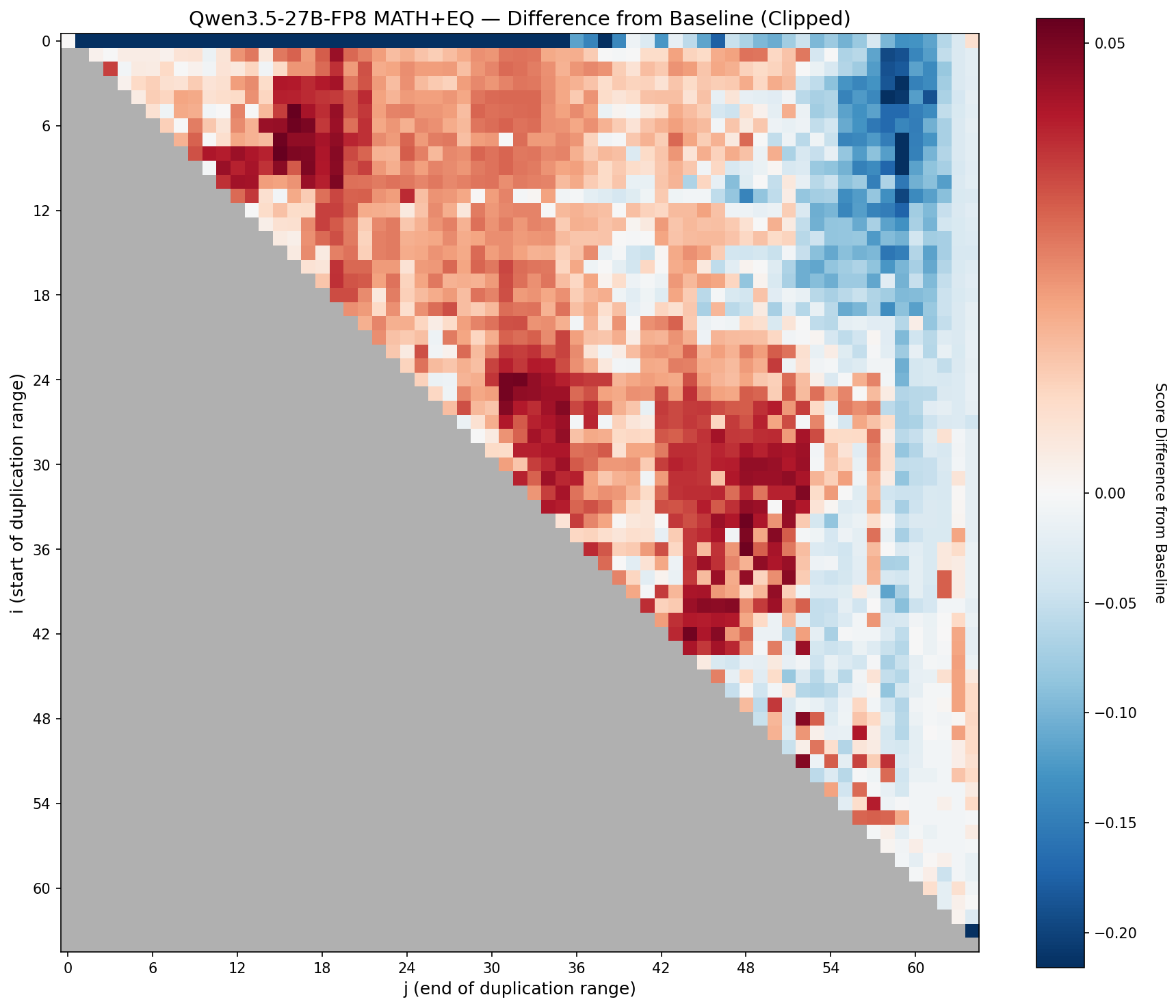
Combined (math + EQ) delta for Qwen3.5-27B. The sweet spot sits clearly in the middle of the stack.
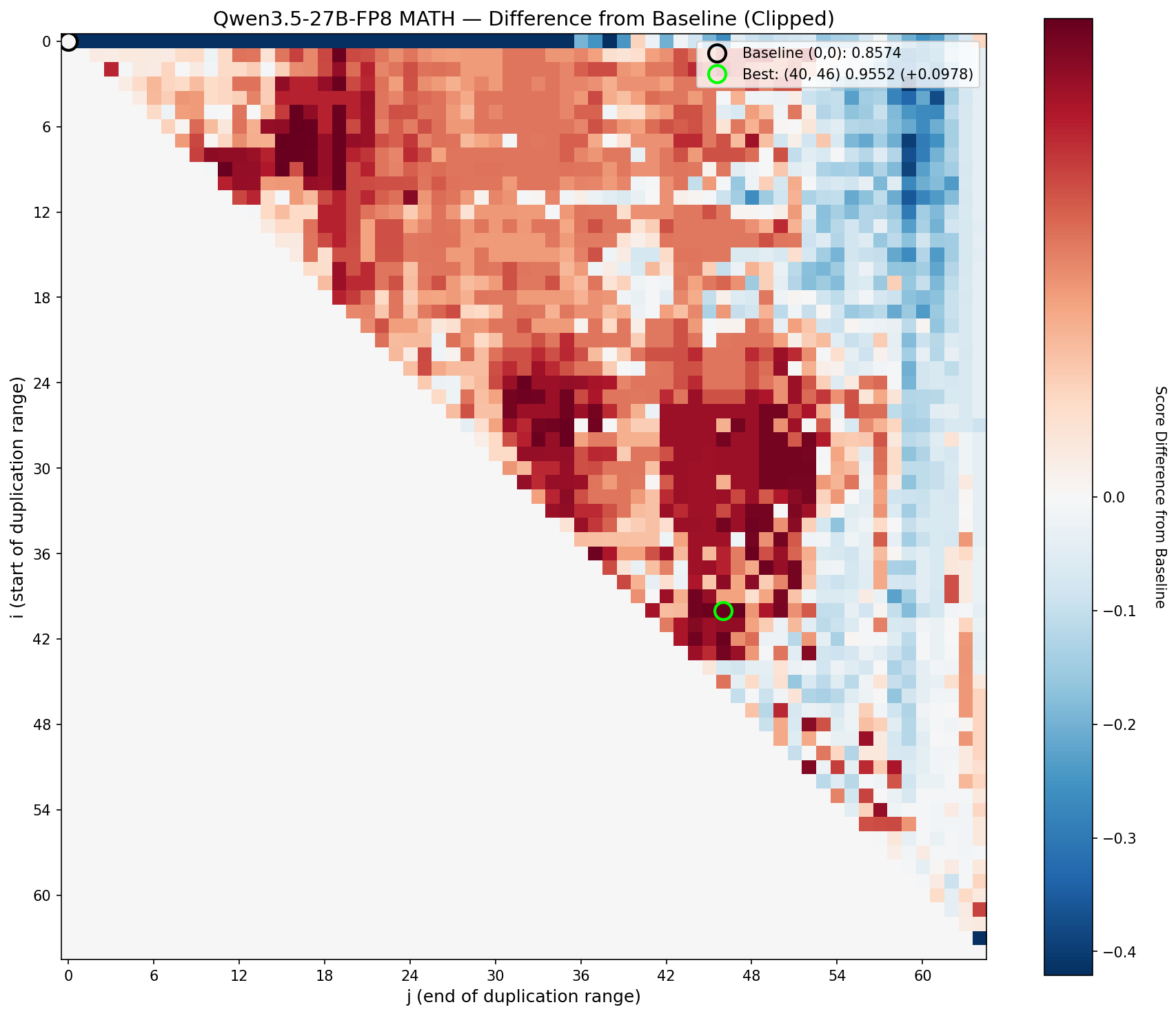
Math delta. Broad mid-stack boost with a clean drop-off at the edges.
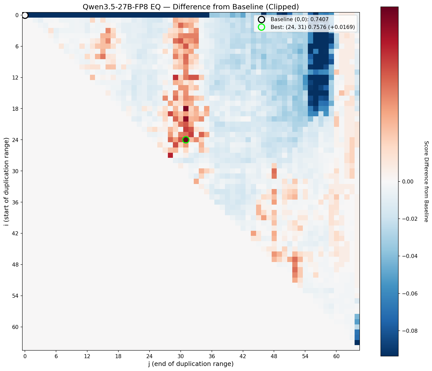
EQ delta. More structured — the useful region is tighter and more sharply bounded.
The signature is pretty clear: even on a modern 27B model, the middle of the transformer stack contains blocks that can be profitably re-traversed. The boundaries are different from Qwen2-72B (as expected, with different architecture, different training), but the general principle holds: there are coherent circuits in the mid-stack, and running them twice makes the model measurably better.
Here are the single-block winners:
| Winner type | Config | Extra layers | Size increase | Math delta | EQ delta | Delta sum |
|---|---|---|---|---|---|---|
| Best math boost | (24,35) | +11 | +17.19% | +0.1203 | +0.0900 | +0.2104 |
| Best EQ boost | (29,34) | +5 | +7.81% | +0.0644 | +0.0975 | +0.1619 |
| Best combined boost | (24,35) | +11 | +17.19% | +0.1203 | +0.0900 | +0.2104 |
The best single block, (24, 35), adds 11 layers (+17% overhead) and boosts both math and EQ substantially. But notice that the best EQ configuration is tighter (just 5 layers at (29, 34)) and gets nearly as good a combined score at less than half the overhead. This is a hint of something we’ll explore a bit later: the efficiency frontier rewards precision over size.
Single-Layer Repeats: Running One Step of the Recipe Again
In Part 1, I showed that repeating a single layer almost never helps. One of the key findings was that the middle layers work as circuits — multi-layer units that need to execute as a whole. Duplicating one step of a seven-step recipe doesn’t give you much.
But “almost never” is doing a lot of work in that sentence. With a stronger model and more compute, I wanted to know if there were any single-layer repeats that reliably moved the needle, and what the profile looked like when you repeated a single layer multiple times.
So I ran a repeat-x8 sweep: for each layer in the 64-layer stack, try repeating it 2×, 3×, 4×, all the way up to 8×. That’s 64 × 7 = 448 configurations, scored against the same math and EQ probes.
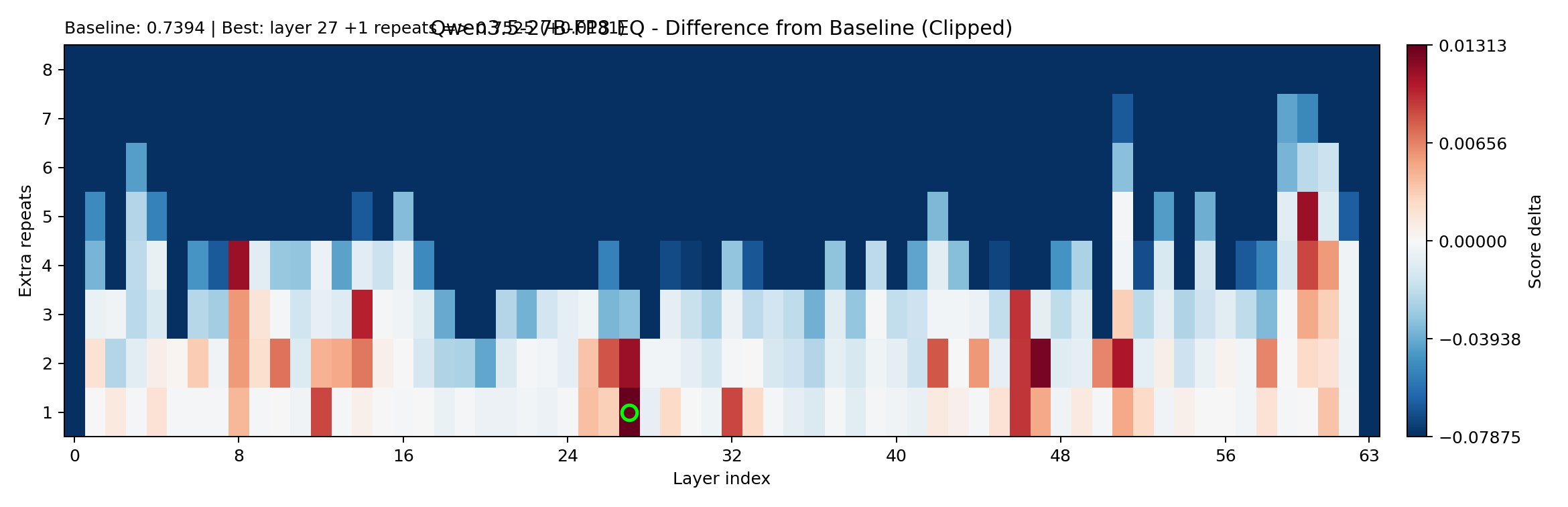
EQ delta for single-layer repeats (x2 through x8). The y-axis is the layer index; x-axis is the repeat count.
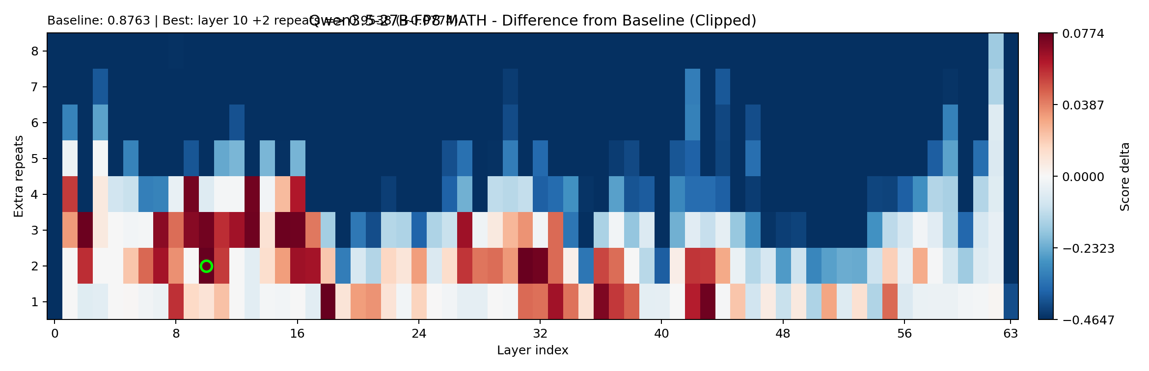
Math delta for the same sweep. Note how different the landscape looks.
The baseline scores for this sweep:
- Math: 0.8763
- EQ: 0.7394
And the winners:
| Winner type | Config | Extra layers | Size increase | Math delta | EQ delta | Delta sum |
|---|---|---|---|---|---|---|
| Best math boost | layer10_x3 | +2 | +3.125% | +0.0774 | +0.0071 | +0.0845 |
| Best EQ boost | layer27_x2 | +1 | +1.5625% | -0.0405 | +0.0131 | -0.0274 |
| Best combined boost | layer10_x3 | +2 | +3.125% | +0.0774 | +0.0071 | +0.0845 |
Two things jump out. First, single-layer repeats can move the model — layer10_x3 gets a solid math boost at minimal overhead. Second, the profile is asymmetric: math can improve significantly while EQ gains are small and unstable. The best EQ repeat actually hurts math.
Beam Search: Composing Blocks
After single-block results, the obvious next question: What if I repeat a block twice? What if you compose multiple blocks? Maybe one block boosts math and a different block boosts EQ, and together they do both.
Brute force is hopeless. Even with just two blocks, the combinatorial space explodes. So I used beam search: start with the best single blocks, then greedily extend by trying all possible second blocks, keep the top candidates, extend again. (This includes of course repeating the same block multiple times, a highly requested feature.)
The beam search parameters:
- Beam width: 24 (keep the 24 best candidates at each depth)
- Starting depth: 3 (begin with the top 3 single-block results)
- Completed depths: 3, 4, 5, 6
- Candidates evaluated: 3,024
- Stopping criterion: 14-hour compute budget exhausted
- Max extra layers: capped at 56 (to prevent absurd configurations where the model is more duplicate than original)
Each candidate was fully evaluated: load the re-layered model, run both probes, record scores. No surrogate predictions at this stage — these are all measured.
Best candidates from the beam search:
| Bucket | Config | Size increase | Math delta | EQ delta | Delta sum |
|---|---|---|---|---|---|
| Best ≤20% overhead | 43,45;28,34 | +12.50% | +0.0978 | +0.1232 | +0.2210 |
| Best overall | 39,45;24,35;9,20;43,46 | +48.44% | +0.1122 | +0.1275 | +0.2397 |
Beam did find stronger absolute deltas than single-block search. The best ≤20% overhead candidate composes two blocks (one in the mid-stack, one higher up), and gets a combined delta of +0.2210, beating the best single block’s +0.2104 while using less overhead (12.5% vs 17.19%).
But beam also made the cost problem obvious. The best overall candidate uses four composed blocks at +48.44% overhead for only a modest improvement over the two-block version. The gains are real but sublinear: you don’t get four times the benefit from four blocks. The circuits interact, and not always constructively. Some combinations cancel out. Others step on each other’s toes.
The lesson: composition works, but it’s not additive. Each additional block buys less than the last, while the overhead grows linearly. For practical deployment, you want the minimum number of blocks that gets you past the performance threshold you care about.
Surrogate Model: Ranking Millions, Measuring Hundreds
Beam search is effective but expensive. Each evaluation means loading a re-layered model and running both probe sets, which takes minutes per configuration. At 3,024 candidates, that’s already pushing the limits of a single overnight run.
To explore the space more broadly, I trained a surrogate model: a cheap predictor that estimates how good a configuration will be, so we can rank millions of candidates and only benchmark the most promising ones.
Training the Surrogate
The idea is straightforward. We already have thousands of measured $(i, j)$ results from the full scan, the beam search, and the repeat sweep. Each measured row is a training example: the configuration parameters go in, the math delta and EQ delta come out. Train a fast model on these pairs, and use it to score configurations we haven’t measured.
I used XGBoost (gradient-boosted trees), which is perfect for this: fast to train, fast to predict, handles the kind of structured tabular features that describe layer configurations well.
Training details:
- Total measured rows: 4,643
- Train/holdout split: 4,411 train / 232 holdout (5%)
- Features: encoded from the configuration spec (which layers are repeated, how many times, block boundaries, etc.)
Holdout validation (Spearman rank correlation):
| Target | Spearman ρ |
|---|---|
| Combined | 0.933 |
| EQ delta | 0.944 |
| Math delta | 0.788 |
A Spearman of 0.93+ on the combined metric means the surrogate is excellent at ranking configurations — which is exactly what we need. It doesn’t have to predict the exact score; it just needs to know that configuration A is probably better than configuration B. The math correlation is lower (0.79), which makes sense: math performance has more noise and depends on subtler features of the block boundaries.
Sweeping 2 Million Candidates
With the surrogate trained, I generated 2,000,000 candidate configurations — spanning single blocks, multi-block compositions, sparse repeats, and various exotic arrangements. The surrogate scored all of them in minutes.
After applying size and sanity filters:
- Candidates scored: 2,000,000
- Accepted after filters: 430,464
- Top candidates fully benchmarked: 100
The top surrogate-ranked candidate that was subsequently measured:
- Config: sparse repeat motif around layers 19/43/51
- Extra layers: +3 (+4.69%)
- Math delta: +0.0328
- EQ delta: +0.0824
- Delta sum: +0.1152
This is interesting — a sparse repeat of just three individual layers, not a contiguous block, that nonetheless produces meaningful gains at under 5% overhead. The surrogate found something the beam search wouldn’t have: a configuration that’s good precisely because it’s minimal.
Important caveat: the surrogate was only used for ranking. Every number in the comparison tables below comes from actual measured runs, not surrogate predictions.
Larger Validation Sets: Graduating from 16 Questions
Up to this point, all the search — full scan, beam, repeats, surrogate — used the original small probe sets: 16 math questions and 16 EQ scenarios. These were designed for speed, and they served that purpose well. But 16 questions is thin for making final claims. A lucky or unlucky draw of questions could shift rankings.
For the final comparison, I built larger validation sets:
Math120: 120 questions with a deliberate mix of difficulty types:
- 60 square root questions
- 30 multiplication questions
- 30 cube root questions
This is more balanced than the original 16, which leaned heavily on cube roots. Different operations stress different aspects of the model’s numerical intuition, and the larger sample size smooths out noise.
EQ140: 139 first-pass EQ-Bench scenarios (the file says 140, but one was filtered during preprocessing — a reminder that data is always messier than you’d like). These span a wider range of social situations, emotional states, and complexity levels than the original 16.
The workflow from this point was:
- Use the small probes for fast search (full scan, beam, repeats, surrogate).
- Shortlist the top candidates from each method.
- Re-measure everything on Math120 + EQ140.
- Compare only the re-measured results.
This means the search phase and the validation phase use different datasets. The small probes found the candidates; the large probes judge them. It’s the same logic as using a validation set you never trained on, and the same reason the original RYS-XLarge result was credible, since I never optimised for the leaderboard benchmarks.
Pareto Punchline
For the final comparison, I took the top 100 candidates from each method family:
- Full scan (contiguous single blocks): 100
- Beam search (multi-block compositions): 100
- Repeat-x8 (single-layer repeats): 97 (a few duds fell below threshold)
- Surrogate-measured (top surrogate picks, fully benchmarked): 100
That’s 397 configurations, all re-measured on the shared Math120 + EQ140 validation sets. Then I computed the Pareto frontier: the set of configurations where no other configuration is both better and smaller.
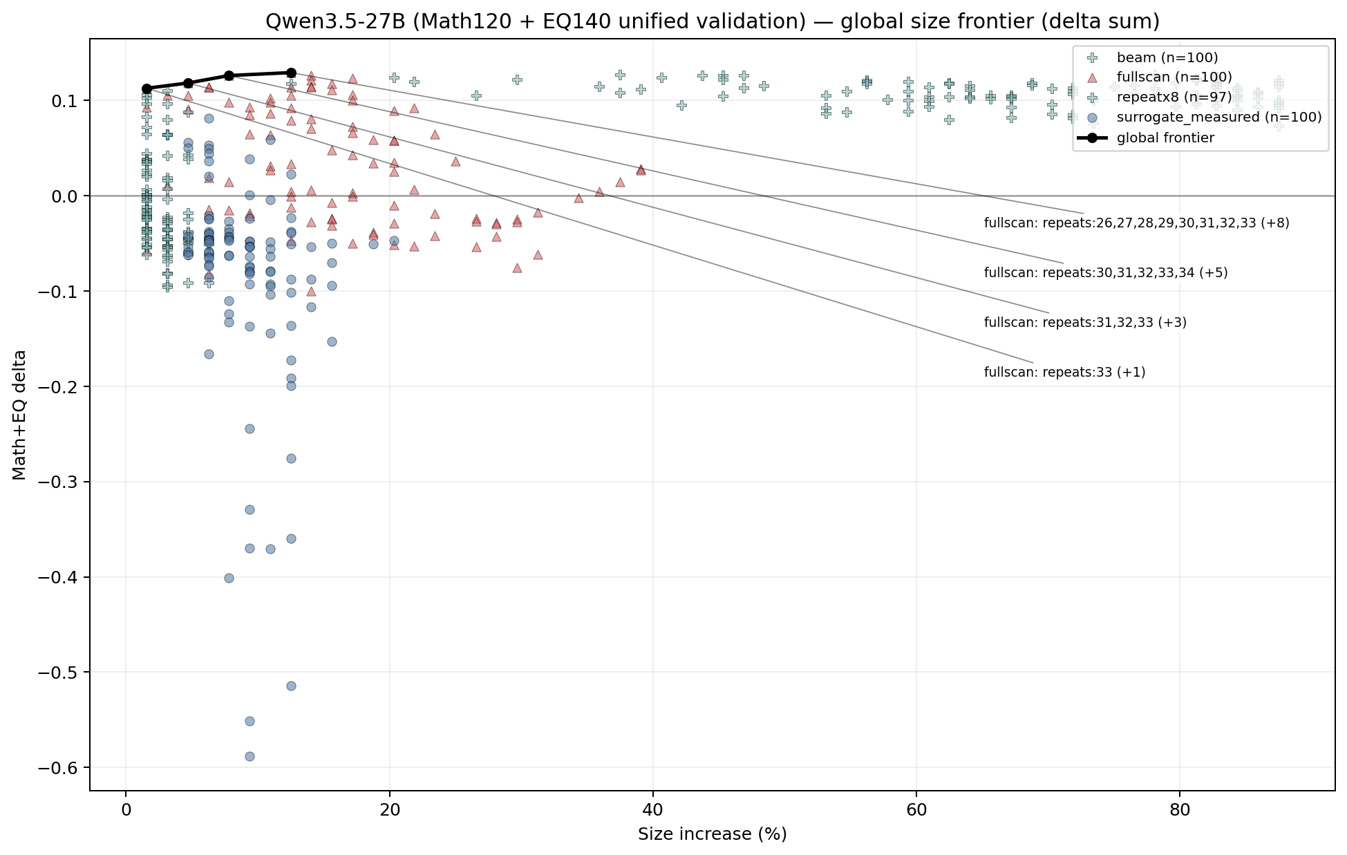
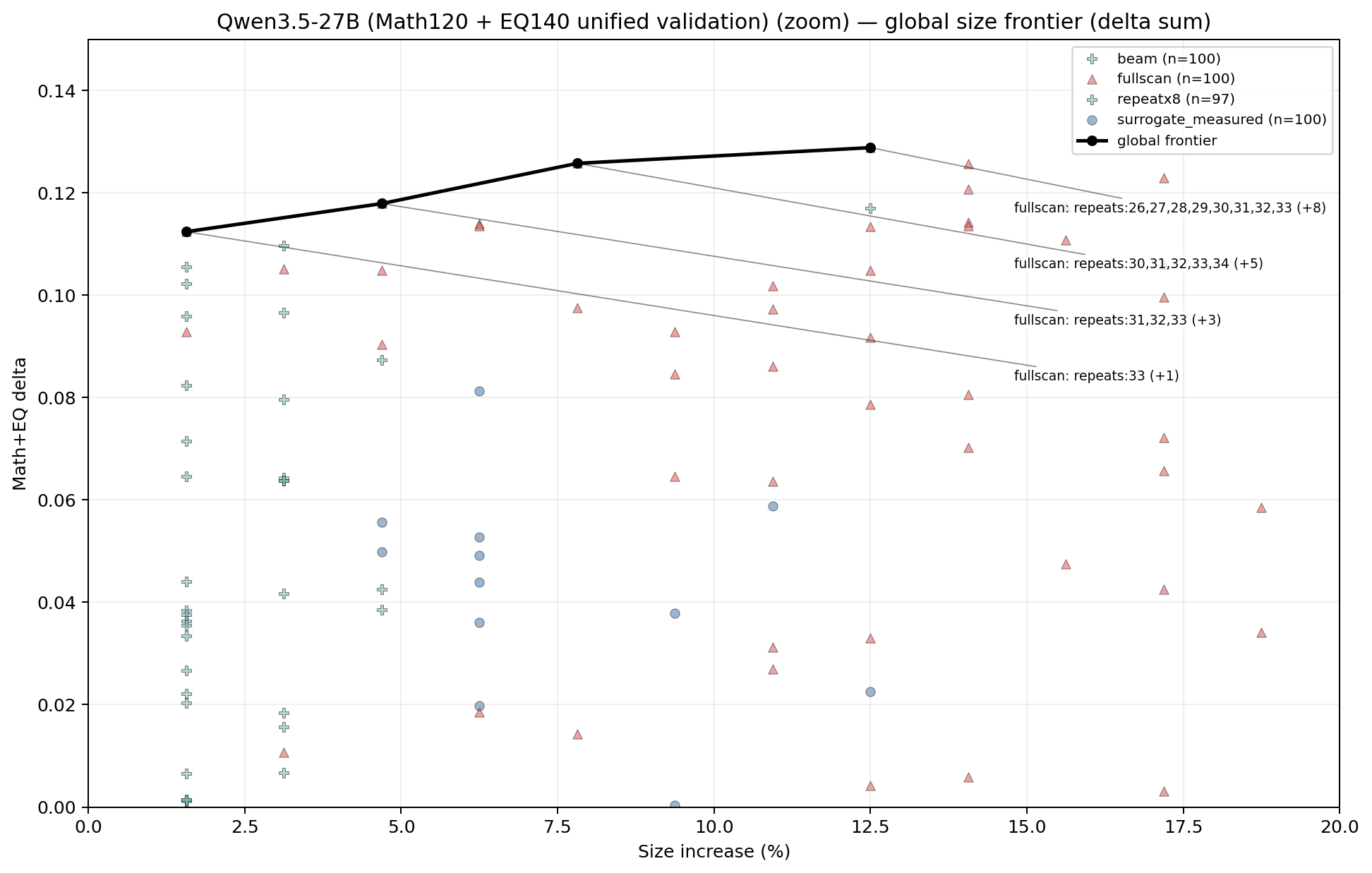
After all that engineering — beam search, surrogate models, 2 million candidates, larger validation sets — the Pareto frontier had four points. All four are from the contiguous-block family:
| Config | Block view | Size increase | Math delta | EQ delta | Delta sum |
|---|---|---|---|---|---|
repeats:33 | (33,34) | +1.5625% | +0.0179 | +0.0945 | +0.1124 |
repeats:31,32,33 | (31,34) | +4.6875% | +0.0207 | +0.0972 | +0.1179 |
repeats:30,31,32,33,34 | (30,35) | +7.8125% | +0.0279 | +0.0979 | +0.1257 |
repeats:26,27,28,29,30,31,32,33 | (26,34) | +12.5% | +0.0279 | +0.1009 | +0.1288 |
This was the key result for me: After throwing every search method I had at the problem, clean contiguous blocks in the mid-stack still dominate the size/performance frontier.
Note: repeating layer 33 alone is both a block AND a single layer repeat, but just saying it’s a block makes the story nicer, ok?
Look at the progression. Adding layer 33 alone gets you most of the EQ boost (+0.0945) at low cost (1.5% more compute). Expanding to layers 31–33 adds a bit more. Going all the way to 26–33 gives the best absolute score, but the marginal returns are clearly diminishing. The EQ delta barely moves from +0.0945 to +0.1009 across a 10× increase in overhead.
This is exactly what the circuit hypothesis predicts. There’s a core computational unit somewhere around layers 30–34 that performs a complete reasoning operation. Duplicating it gives the model a second pass through that operation. Making the block larger captures some neighbouring context, which helps marginally, but the essential circuit is small and well-defined.
Notably absent from the Pareto frontier: multi-block beam compositions and exotic surrogate picks. They can produce strong raw scores, but they do it at higher overhead than a simple contiguous block achieves for the same benefit. Complexity doesn’t pay on the efficiency frontier. That said, it would probably be amazing for model expansion and continued fine-tuning. You have already prepared the model by adding the right kind of layers to refine ‘thinking’, and I think this is a via model for Frontier Labs to play with (and if not, sponsor me with some Nvidia gear at least).
The Models
With the analysis complete, I built the RYS variants and uploaded them to HuggingFace. These use the Pareto-optimal configurations from the table above.
S is for people who want the maximum EQ boost at near-zero overhead. Play around with M and L to find your preferred best balance of performance and cost. XL is for when you have the compute and want the strongest absolute scores.
These are regular HuggingFace weights, but I’ll be working with TurboDerp to build Exllama v3 models with pointer-based layer duplication: the repeated layers share weights with their originals. No additional VRAM is consumed for the parameters themselves — you only pay extra for the compute time and KV cache of the additional forward passes. This means you can run RYS-Qwen3.5-27B on the same hardware that runs the base model! Stay tuned…
As discussed in Part 1, I believe the junction points (where the model loops back to an earlier layer) are the main source of residual inefficiency. A LoRA fine-tune targeting just those junction layers should further improve performance without converting the pointer-based duplicates into real copies. I haven’t done this myself, but if the Qwen2-72B pattern holds, the community will take it from here.
The Code
The scanning pipeline, probe datasets, and model-building scripts are available at:
The repo contains:
- Scanner: the $(i, j)$ sweep pipeline, including the math and EQ probe evaluation harnesses
- Probes: all datasets used in this work (math_16, math_120, EQ_16, EQ_140)
- Beam search: the multi-block composition search
- Surrogate: XGBoost training, candidate generation, and top-k benchmarking pipeline
- Model builder: scripts to produce RYS variants from any HuggingFace model given a configuration spec
- Heatmap generation: plotting code for the brain scans
The core dependency is ExLlamaV3 for quantized inference. Most of the scanning was done with FP8 quantized models, which fit comfortably in the 192GB HBM3 on my Hopper system. For the original Qwen2-72B work, I used ExLlamaV2 on dual 4090s — the pipeline works on consumer hardware, it just takes longer.
What This Means
For Qwen3.5-27B specifically:
- If you want low overhead and reliable gains, a single contiguous block in the mid-stack is still the best first move.
(33, 34)gives you most of the benefit for almost nothing. - Sparse single-layer repeats are real and useful as low-cost alternatives, especially for math-heavy workloads.
- Composing many motifs can produce strong raw scores, but overhead climbs fast and the interactions are sublinear.
- The Pareto frontier is clean. Contiguous blocks dominate once you account for size.
More broadly, this work confirms what Part 1 suggested: Transformer reasoning is organised into discrete functional circuits, and this organisation is a general property, not an artifact of one model or one generation of models. The circuits are there in Qwen3.5-27B, just as they were in Qwen2-72B, Llama-3-70B, and Phi-3. The boundaries differ. The principle doesn’t.
The method is orthogonal to fine-tuning, orthogonal to quantisation, and orthogonal to whatever prompt engineering you’re doing. It’s a free lunch, or at least a very cheap snack. The model gets smarter by thinking longer, using the reasoning circuits it already has.
More architectures are in the pipeline. The Hopper is still grinding on MiniMax M2.5. Watch this space!
Citing this work
1
2
3
4
5
6
7
@article{ng2026rysii,
  title   = {LLM Neuroanatomy II: Modern LLM Hacking and hints of a Universal Language?},
  author  = {Ng, David Noel},
  year    = {2026},
  month   = {March},
  url     = {https://dnhkng.github.io/posts/rys-ii/}
}