Differential geometry has a reputation as something that
many non-mathematicians want to learn (e.g., it is very relevant to physics, particularly general relativity), but
is so expansive and in parts arcane that it is difficult to know where to start.
To give you an idea, the only reasonably well-known textbook that I could find treating differential geometry at an undergraduate level (and, mind you, this is meant for the last couple of years of a mathematics undergraduate major) is Pressley’s Elementary Differential Geometry, which:
is about 400 pages long,
leaves out far more than it includes, and
still has many reviewers complaining about it being difficult to read.
I don’t know if it is really possible to teach differential geometry to an undergraduate audience and do the subject (or your students) much of any justice. But let’s set a much lower bar: let’s do a rough overview of differential geometry. We’ll discuss what the basic constructions of interest are, and what sort of things you might want to do with them. This should give the reader an idea of what to look for if they want to study it further.
Let’s begin with differential topology, since that is the bedrock on which all differential geometry rests, and some even consider it to be a part of differential geometry itself.
The basic structure of differential topology is the differentiable manifold. To build a differentiable manifold, you start with a topological manifold. Intuitively, this is a space such that sufficiently small pieces of it look Euclidean. Here’s the formal definition.
Definition: A topological manifold is a second-countable, Hausdorff, topological space M such that for every point p on M, there exists some open neighborhood of p that is homeomorphic to an open neighborhood of ℝn. (For some fixed, non-negative integer n: this is called the dimension of the manifold.)
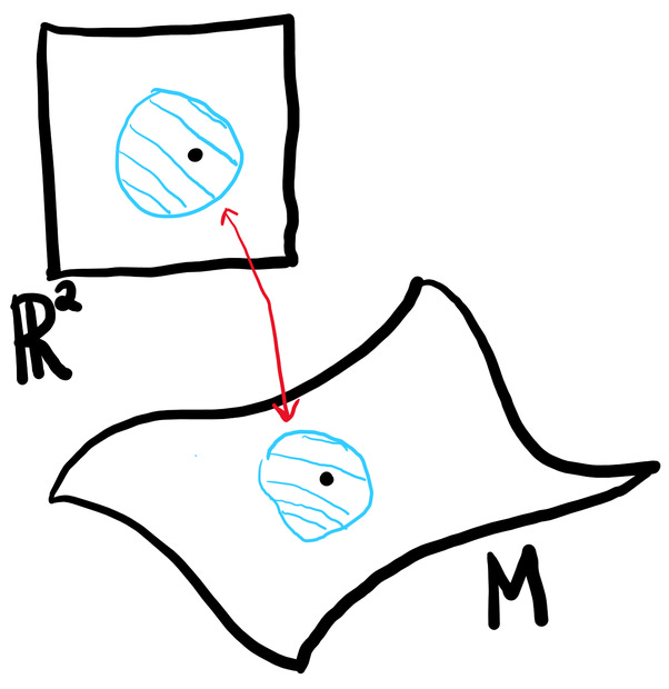
If you are unfamiliar with topological spaces, you should focus on having a picture like the above in your head. The idea of a topological space is that it allows you to define what a continuous function is. So what we are asking is that, for any sufficiently small region around a point of this manifold, there exists a continuous function with a continuous inverse from this region to a region of ℝn. We need a couple of additional technical requirements (it must be second-countable, Hausdorff), which are there to weed out any pathological examples.
A circle is a good example of a topological manifold.
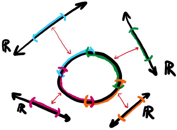
So would be any other (non-self-intersecting) curve, the sphere, the torus, the Klein bottle, and so on.

Topological manifolds are very important in topology, but they are much too limited for our purposes—they allow you to reason about continuity (and therefore connectedness, compactness, and other topological notions), but they lack any notion of differentiability. To oversimplify it a little, there’s no way to define what a “corner” or a “cusp” is for a topological manifold. So, for instance, both the disk and the square are essentially the same topological manifold: you can continuously deform one into the other. But the square has corners while the disk does not.
How to capture such a difference? This is where differentiable manifolds come in.
Definition: A differentiable manifold is a topological manifold M of dimension n together with a collection of compatible charts that form an atlas. A chart is an open subset U of M together with a homeomorphism τ: U→U′, where U′ is an open subset of ℝn. Given two charts (U, U′, τ1), (V, V′, τ2), we say that they are compatible if the transition map

is differentiable. A collection of charts is called an atlas if every point in M is contained in some chart—that is, the charts cover all of M.
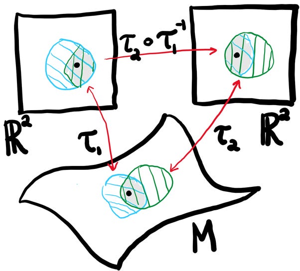
Let’s pause just a second to digest what the hell that is saying, and why it matters. We said previously that for a topological manifold, there is an open neighborhood around each point that is homeomorphic to an open neighborhood of ℝn—that’s what a chart is.
Now, let’s say that we want to define what it means for a function f: M→ℝ to be differentiable. If M were ℝn—or, more generally, an open subset of ℝn—we would know how to make sense of that. So, we might try to make clever use of the fact that we have charts: define f: M→ℝ to be differentiable at a point p if, when we take a chart (U, U′, τ) with p in U, the function f∘τ−1: U′→ℝ is differentiable. The idea is that the chart allows us to essentially identify U and U′, but U′ is actually an open subset of ℝn, so all is well.
Or is it? There’s a problem with what I have just said, because this point p will necessarily be contained in multiple charts. Could it happen that a function f is differentiable at p if we choose one such chart, but not if we choose another?
If we imposed no conditions on the charts, then, yes, that absolutely could happen! Let’s suppose that we have two charts (U, U′, τ1) and (V, V′, τ2) which overlap: that is, U∩V1 is not empty, as in the drawing I had above. Then we have a transition map

What is this? The idea is that the image of U∩V appears in both U′ and V′, and so we have a homeomorphism between them. That is why it is called a transition map: it transitions between these two charts.
But it is also a function between two open subsets of ℝn, and so it makes total sense to ask whether it is differentiable or not.
Now, suppose that it isn’t. Then we have a little bit of a problem, because

So, if this transition map isn’t differentiable, then it could easily happen that f∘τ2−1 is differentiable, but f∘τ1−1 isn’t (since it is the composition of a differentiable and non-differentiable function).
Conversely, if the transition map is differentiable, then we are fine: one will be differentiable if and only if the other one is! This is why we say that the transition map is compatible if it is differentiable: it allows us to define differentiability in such a way that it is compatible across different charts. And if the charts cover the entire manifold—meaning that they form an atlas—then we have a notion of differentiability that works across the whole thing.
The names here are deliberately evocative. If you take an atlas of the Earth, it will consist of a collection of charts: flat maps that cover a portion of the entire surface. As long as you are traveling within the area covered by a single chart, everything is fine, but if you need to travel beyond that, you need to understand how one chart transitions to the next in the place where they overlap.
Let’s discuss some of the things that a differentiable manifold allows you to define (which would not make sense for a mere topological manifold). To start with, given two differentiable manifolds M, N, we can define a function f: M→N to be differentiable if for every point p in M, if we choose a chart (τ1, U, U′) of M that contains p and a chart (τ2, V, V′) of N that contains f(p), then τ2∘f∘τ1−1 is differentiable.
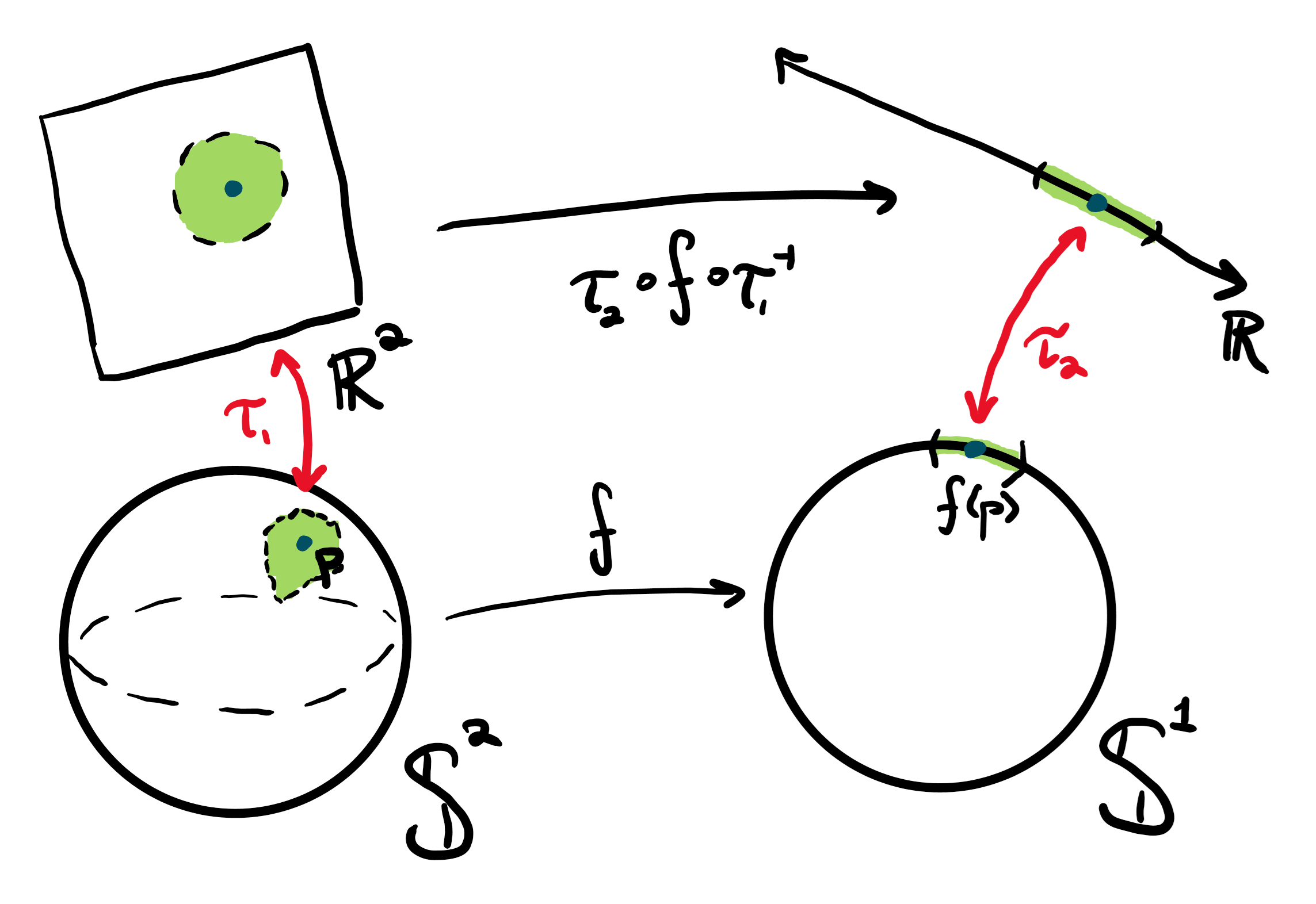
Here is an example of how this might look. I could take the unit sphere 𝕊2 and the unit circle 𝕊1—these are both naturally differentiable manifolds2. And then I might have some function like

and to determine whether it is differentiable or not, you would need to write it down using the charts to get a function ℝ2→ℝ for which you can check differentiability.3
The next big thing that you can define on differentiable manifolds is vector fields. Unfortunately, this is a bit complicated because there is a bit of a disconnect between how you would naively want to define vector fields and how you actually do it in practice. You’ll see what I mean in a second.
You want to define vector fields on differentiable manifolds by picturing little arrows tangent to the curve/surface/hypersurface, like in the following illustration.
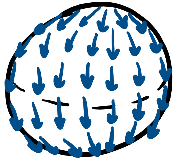
But where do such arrows live? It isn’t inside the manifold itself—it would have to be in some ambient space. Now, it does turn out that any differentiable n-dimensional manifold can be realized as some subsurface in ℝ2n. But there are many issues with this approach:
Showing this isn’t exactly non-trivial—it was proved by Whitney in the 1930s.
It is inconvenient: while you can realize, say, the Klein bottle as a subsurface of ℝ4, I don’t think I have ever actually seen anyone do it, because it is an ugly and unintuitive representation.
There are many ways to represent differentiable manifolds as subsurfaces of Euclidean space, so you would have to argue that the particular representation doesn’t actually matter.
Even if you do have some nice, canonical embedding in Euclidean space (like, say, the sphere has), you’ll still need to define what it means to be tangent to the manifold somehow. It can be done, but it isn’t all that clean.
So what can you do instead? There are quite a few equivalent definitions; since we are not burdened by a need to carry out explicit computations, I’m going to give the one that I feel is the most visual/easy to comprehend.
Definition: A differentiable curve on a differentiable manifold M is a differentiable function γ: ℝ→M.
We’re going to define what we mean by a vector at a point p in M in terms of differentiable curves.
Definition: Choose a point p, a chart (τ, U, U′) that contains it, and consider the collection of differentiable curves γ such that γ(0)=p. We’ll say that two such curves γ1, γ2 are equivalent if

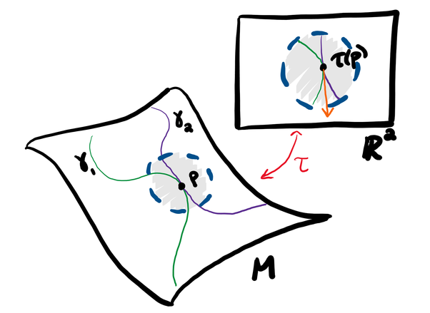
What is the idea here? The images of these curves in the chart (that is, in ℝn) have the same tangent vector. Note that this doesn’t depend on the particular chart used: it is actually a property of the curves. So, what we can now do is define vectors at a point via tangent vectors to a curve. This gives us the following definition.
Definition: Let M be a differentiable manifold. Let p be a point of M. The tangent space TpM of M at p is the collection of equivalence classes of differentiable curves γ: ℝ→M such that γ(0)=p.
What you then show is that TpM has a natural structure as a real vector space—specifically, it will be isomorphic to ℝn.4 It’s not very difficult; the easiest approach is to note that, without loss of generality, you may assume that τ(p)=(0, 0, 0,…, 0), since translations are differentiable and so, at worst, you’ll get a different but compatible chart. This allows us to define what a vector field on M is.
Definition: A vector field on a differentiable manifold M is a continuous function that takes points p in M and returns vectors in TpM.
How can we define continuity here? Here’s a fairly simple way: if you want to check continuity at p, just use a chart (τ, U, U′) and observe that your function can now be considered a function U′→ℝn, and we know exactly what it means for such a function to be continuous.
Given any differentiable function f: M→N between two differentiable manifolds, we can (and should!) ask about what this function does to vectors, as follows: choose some specific differentiable curve γ: ℝ→M that represents your vector in TpM. Then f∘γ will be a differentiable curve such that (f∘γ)(0)=f(p), which is to say that it represents some vector in Tf(p)M. One checks that this vector does not depend on the particular γ used.
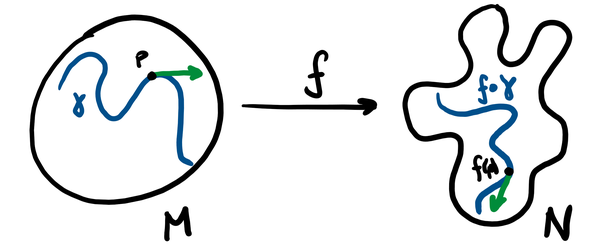
As a result, we get a map Dpf: TpM→Tf(p)N, known as the differential of f at the point p—this extends, of course, to a map Df that maps every vector at p in M to a vector at f(p) in N. One checks that the differential at a point is, in fact, linear—that is,

The differential comes up often in computation, often referred to as the Jacobian. But there is a special case that is more important for our purposes, which is what happens in the case where N=ℝ. In that case, we can naturally think of Tf(p)N as simply being ℝ, which means that Dpf—usually simply written as df in this context—is a linear map TpM→ℝ.
Definition: The collection of all linear maps TpM→ℝ is called the co-tangent space of M at p, and is usually denoted by Tp∗M. An element of it, such as df, is called a co-vector. A continuous function that takes points p in M and returns co-vectors in Tp∗M is sometimes called a co-vector field, but more commonly it is called a 1-form.
We have already produced the prototypical example of a 1-form: take any differentiable map f: M→ℝ and its differential df will be a 1-form.
Okay… but, intuitively, what the hell is a 1-form? And why is it something useful? Arguably, the answer to both of these questions is the same: a 1-form is something that you can integrate over an oriented curve. (Oriented here means that you keep track of where the curve starts and where it stops. If you integrate in the opposite direction, the sign flips.) If you ever encountered a line integral (in multivariable calculus or physics, for instance)

that is precisely an example of a 1-form on ℝn, integrated over some curve. Specifically, the 1-form is

where

Then, as we saw previously, dxi is a well-defined 1-form, and it isn’t hard to see that if ω1, ω2 are 1-forms and f, g: M→ℝ are differentiable functions, then fω1+gω2 will also be a 1-form—thus, the expression above really is a 1-form.
The general theory of how you define the integration of 1-forms, how to actually compute them, and how to do coordinate transformations, is somewhat involved, and so I am going to skip it here.5
Of course, if a 1-form is something that you integrate over an oriented curve, then the next natural question is what sort of object would integrate over an oriented surface/volume/hyper-volume? The answer to that is that you need differential forms, but we’re going to define something a bit more general.
Definition: Choose a point p on a differentiable manifold M. A tensor at p is a multilinear function (TpM)m×(Tp∗M)n→ℝ. That is, it takes in some number of vectors, some number of covectors, and returns a real number, with the stipulation that it must be linear in each of its m+n inputs. We will denote the collection of tensors at p by Γp(M, m, n). A tensor field is a continuous map that takes in points p in M and returns tensors in Γp(M, m, n).
Vector fields and differential forms are just special kinds of tensor fields. In fact, a lot of things in differential geometry are just special kinds of tensor fields, or in some way derived from tensor fields. (For example, unsigned volume, surface area, and arclength are almost tensor fields, because they have an additional corrective factor.)
I think that is enough of an introduction to the basic objects in differential geometry. Let’s move on to going through various branches of the field. All of them build on the basics of differential topology exposited above, but with some additional structure added that allows us to talk about something like length or angles or volume, etc., etc.
For example, when we defined differentiable manifolds, we specified that two charts were compatible if the transition maps were differentiable. Instead, we could impose some kind of stronger condition. For example, if our manifold is 2-dimensional, we can interpret the chart as mapping to an open subset of the complex numbers ℂ, and in that case, it makes perfect sense to require that the transition maps aren’t just real differentiable, but complex differentiable (i.e., holomorphic). You can generalize to the case where the manifold is even-dimensional—this gives rise to the notion of complex manifolds.
Complex manifolds are more structured than differentiable manifolds, because while holomorphic maps don’t have to preserve any kind of distance, unlike differentiable maps, they do have to preserve angles and orientation. Below is an illustration of a holomorphic transformation between the open disk and the half-plane, both interpreted as complex manifolds. You can see that distances get distorted, but angles between curves are preserved.
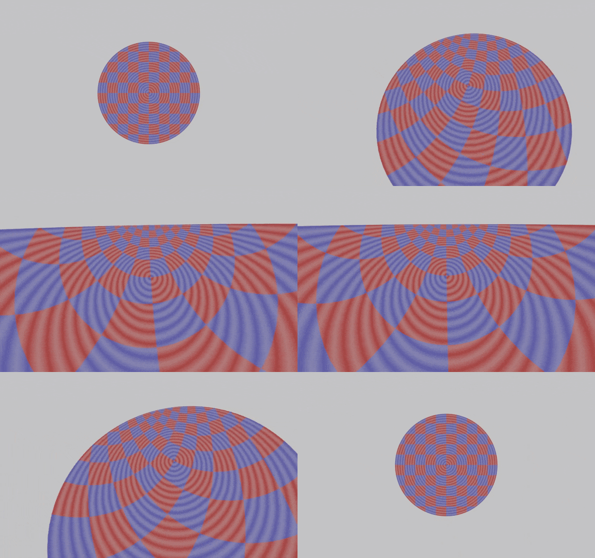
Another option is to introduce some kind of tensor field on your differentiable manifold—you can then study transformations that preserve this field in some fashion. Let’s illustrate a few examples.
Definition: A Riemannian manifold is a differentiable manifold M together with a tensor field on M such that at every point p in M, the corresponding tensor is a positive definite bilinear form on TpM, known as the Riemannian metric. That is, the metric is a bilinear map gp: TpM×TpM→ℝ such that

The idea is that this form acts like the normal dot product on ℝn—it allows you to define the lengths of vectors in TpM as well as angles between pairs of vectors. But this immediately means that we can define something like the arclength of a differentiable curve γ: [a,b]→M: it will just be

where γ̇(t) is the tangent vector of γ at γ(t) in Tγ(t)M. If M=ℝn and gp is just the standard dot product, you can see that this reduces to the standard formula for the arclength of a curve.
Of course, once you have a notion of distance, you get all of the other hallmarks of geometry: area, volume, and so forth. Unlike differentiable manifolds or even complex manifolds, Riemannian manifolds are very rigid.
A related generalization is the pseudo-Riemannian manifold, which gained a lot of prominence due to its connection to general relativity. A pseudo-Riemannian manifold differs only in that the bilinear form is only required to be non-degenerate and not positive-definite—that is, one must change condition (2) above to the following:

The simplest pseudo-Riemannian manifold that is of much interest is Minkowski space: this is just ℝ4, but the pseudo-metric is

This doesn’t allow you to define distance per se—instead, it allows you to define what is known as the space-time interval.
There are various other examples where you start with a differentiable manifold and then add on some canonical tensor field—in symplectic geometry, one adds a differential 2-form instead. This also has applications in physics (it is a natural way to represent phase space), but I must admit that I know next to nothing about it other than the fact that it exists.
Here’s one more completely different way to add structure to a differentiable manifold: give it a group structure! Specifically:
Definition: A Lie group is a differentiable manifold M together with two differentiable maps ⋅: G×G→G and ∗−1: G→G such that the following conditions are met:
⋅ is associative: that is, a⋅(b⋅c)=(a⋅b)⋅c.
There exists an element 1 in G that is the identity: that is, 1⋅a=a⋅1=a.
Every element has an inverse: that is, a-1⋅a=a⋅a-1=1.
The classic example of a Lie group is GL(n, ℝ), the collection of invertible n×n real matrices, which we covered numerous times in the group theory notes. It has a natural interpretation as a differentiable manifold (it is a subset of ℝn×n) and matrix multiplication and inversion have the desired properties. There are countless others, although Lie groups are even more rigid than Riemannian manifolds—so much so that there is a classification of them. On the other hand, they are incredibly useful in mathematics, physics, and beyond (e.g., they have been studied in the context of computer vision).
So that’s the quick crash course in differential geometry. I can barely be said to be scratching the surface, but I hope it gives the reader enough to seek out what they need/want.