Welcome to Part 4 of a series on language modeling. In Part 3, we got familiar using vanilla RNNs for the next-character prediction task. We saw the main advantage of adding recurrence to the network is to keep track of long-term dependencies in the input stream. For example, predicting the closing quote in
John said, “I can’t make it to the gym today because I have to work”
requires the model to remember the opening quote at the beginning. Recurrence allows the model to remember previously seen tokens so that it can consider them for the current prediction.
This is the sample story from the latest model:
Story time: Once upon a little eazings ont Day, I kidgo preate it said. At and you were ittlied. The dreing frien fell backy. She is a camed an. Dadry, Tommy said, “Now, Timmy. He good they fate ause wime caplo. Shew it a with and purnt wike to na;e and hoar. Her and it was he a wourhan. Bobse time, tak mom in the mom togetecide is the bout his mommy, they prele big to think. The rail a citcus but the ponf the she friendsn. The finger ick will and do sturted the tallo!” Biknywnedded usever,o gand and ce oven tore, girl flew the parn.
Obviously still not performing very well.
The problem with the vanilla RNN is that the recurrent hidden state leads to instability during training - gradients tend to vanish or explode. This instability led to the development of initialization techniques that ensure the hidden weights have a principal eigenvalue of 1. This somewhat helps prevent the gradient problem, however due to numerical drift over long sequence lengths and other terms in the gradient, gradients as a whole still have propagation issues.
This motivated the development of alternative architectures which allow for better gradient flow through the sequence. In this post we will look at the most prominent recurrent successor1 to the vanilla RNN, the long short-term memory (LSTM).
Both RNNs and LSTMs have a hidden state h_t. The hidden state evolves over the sequence dimension, and represents the model’s output at the end. In order to track long term dependencies, the LSTM adds a new state element called the memory cell (or just cell for short, denoted c_t).
The terminology here was confusing to me when I learned this. The cell c_t is completely internal to the LSTM block, so in a sense it is completely hidden. The hidden state h_t is updated internally and eventually output from the model, so in a sense the hidden state is quasi-hidden.
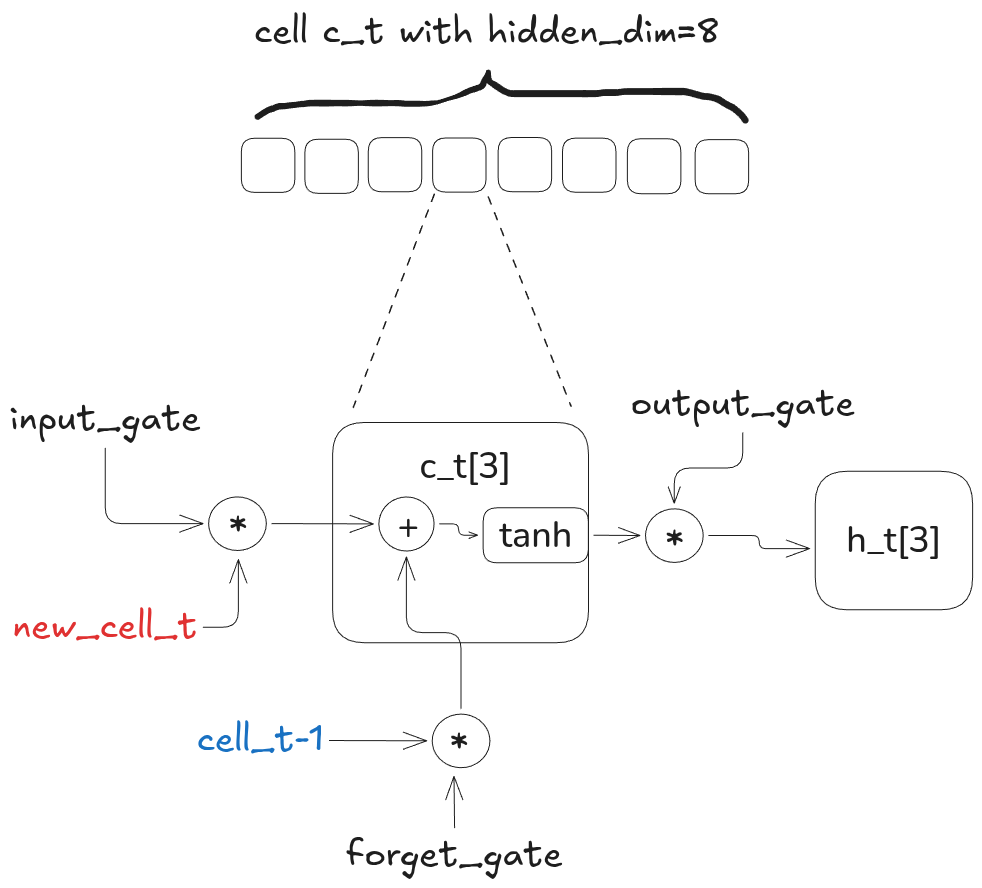
You can think of the cell as a chunk of volatile RAM. Each element in the cell is a hidden unit that can be read from, written to, and reset to zero, analogous to DRAM. These operations are controlled via the output gate (read), input gate (write), and the forget gate (reset). Each of these gates is implemented with a sigmoid non-linearity to provide a differentiable operation of a binary choice.
When the input gate is 0, the cell is effectively ignoring the current token. When it is 1, the cell is prioritizing the current token. The forget gate is “active low”. When it is 0, the previous cell state is forgotten; when it is 1, the previous cell state is remembered. The output gate controls the degree to which the internal cell state is “released” into the hidden state h_t as output.
The other key ingredient that enables the LSTM to keep track of long-range dependencies like quotes, braces, etc. is to feed the hidden state into the gates. The hidden state provides the historical context the gates need to encode state like “we are currently inside a double quote”.
Take the following string:
The writer said, “you need to use double quotes more.”
Consider what the input and the forget gates need to do for a hidden unit in the cell that tracks quotes. At the first quote, the input gate needs to saturate to one and the forget gate needs to saturate to zero. This effectively latches the “inside quote” state representation into the particular hidden unit in the cell. Further, the output gate needs to saturate to one, so that the hidden state encodes “inside quote”. Then for the subsequent characters, this hidden state is fed into each of the three gates, effectively encoding a state transition to “inside quote”. For the non-quote characters, the input gate now saturates to zero and the forget gate saturates to one (i.e. to keep the hidden unit cell state the same). The output gate is still saturated to one to preserve the hidden state. Finally, once the closing quote arrives, the input gate transitions towards one and the forget gate resets towards zero. This transitions the cell’s hidden unit to “outside quote” again, which is fed through the output gate into the hidden state.
Now you may be wondering, what is the point of creating this new cell state? Why can’t we just use the hidden state as in the vanilla RNN?
The reason is that the LSTM construction enables better gradient flow backwards through the sequence dimension. To see why we can look at the code snippet around the cell calculation (you can find all the code for this post here):
# LSTM forward pass function
def __call__(self, x, h=None, c=None):
    ...
    new_cell = torch.tanh(batch @ self.W_xc + self.hidden @ self.W_hc)

    # (1) cell is child of sum operation
    self.cell = f * self.cell + i * new_cell

    # (2) cell is child of non-linearity tanh
    self.hidden = o * torch.tanh(self.cell)

    y = self.hidden @ self.W_hy + self.b_y
    outputs.append(y)
    ...
You can see there are two instances of cell on the right-hand side. This means the gradient of the loss with respect to cell will ultimately be a sum of two terms. The second instance is similar to the calculation of the hidden state in the vanilla RNN in that it is a child of the tanh in the computational graph. The first instance is the critical part, as it is the child of an addition. Since addition directly distributes gradients, this provides an alternative route for gradient to flow to cell across the full sequence dimension. This route provides a bypass around the potentially saturating tanh non-linearity.
Let’s train the LSTM to compare with the vanilla RNN. Note that I added an instance of the Adam optimizer in the training loop. This was used to train both the RNN and LSTM with a sequence length of 32 and hidden dimension of 256. Adam is outside the scope of this post, but I highly recommend reading Why Momentum Really Works in case you are curious to learn more.
The RNN ended with a loss of 1.058 and perplexity of 2.86. This means simply adding Adam provided roughly 33% improvement in the loss and 25% improvement in perplexity!
The LSTM ended with a loss of 0.9177 and perplexity of 2.45. So even with a fairly small sequence length of 32, the LSTM outperforms the vanilla RNN.
Here is a sample story from the RNN:
Story time: Once upon a time, there was a little boy named Timmy. You don’t move. And he reached the grass her toys.
“Of cou did not know. She wants to go home back in the cells. They did it was too enter and said, “No,” Ben got angry angry. Sarate was so happy. They be okay. You are wrong cricket. The bott. She saw lots of lion teaches lesson to have a big bed and a big numbers. They liked to lay.
One day, she watched and said, “That was a room, Ben looked zigingly. The moral of toys and decided to live energe.”
Lily got theard something scarf.
Now that is much better. We can see most of the words are valid English, though still a few that aren’t. We can also see that the model has learned order and structure of quoted phrases in relation to the subject that is saying them.
Here is the LSTM:
Story time: Once upon a time, there was a small bird playing tight he would always made a mess.
Suddenly, their mom smiled and said, “No, new and how to urge her mom. She did not want to send it in his room. He wanted to play in the park with.
Aman was so happy that Lily was walking in the park. She wondered why he was old twigs, but one day it said. “Okay, but you are curious. She went to recorded his wings and answer. Afterwards, he shouted on the way. They do not know that a cupboard before in the bench. Tim determined to quarrel have seen the water. Then asked her dad, “I’m sorry, Ben,” Ben says.
“F’m cool!” She wished he tried to talk to the store and put some strong store on a piece. He played in
This one is even better! All the words except for “F’m” are valid. Now the story still doesn’t have much coherency, but the structure of the story is much better. The main issue is the subjects are coming and going with no real connection to an underlying narrative. Keep in mind that this LSTM used a sequence length of 32 for training. If we want to have coherency across larger portions of the text, perhaps we should have a longer sequence length to capture longer range dependencies.
When we re-train with a sequence length of 128, the loss drops from 0.9177 to 0.8285 and perplexity decreases from 2.45 to 2.32. Here is a story:
Story time: Once upon a time there were two fearful of many toys. They do not notice their fight. They liked to give the chimding into his room. There, they had a doll, I cut the brush to go away. Let’s decide it rown in your bones and your bike, Ben. You are brave and selfish.” They ask Mom and Dad.
“Go?” Lily said, pointing at the balloon. She hugged the doll bitter. She opened her around with her window. One day, she noticed something giragain and the airport. The little bird flew away, curious, and told her family for being so much fun.
Timmy felt happy with his game and went to her mom and stayed because no one wanted to see the flower. Lily realized that being happy she and Lily, was very surprise
It seems performance is roughly the same - the quality of the stories are within the same neighborhood. Most of the words are valid, but the coherence is still lacking.
One more thing we can do is stack LSTMs into multiple layers. In this stacked arrangement, the hidden state outputs for the first layer are fed into the input of the second layer.
The loss from a 2-layer LSTM drops down to 0.7964 with perplexity 2.22. Here is a story sample:
Story time: Once upon a time there was a hunter. She liked to put away them in her little kitten. On the beach winter and was walking home, there were many fish!
Jack made sure to keep him available felt feeling helpless and sparkly, treat, and was getting tracks. The post was the most long in the wheel said, “Thank you should never have to stay up for a while. What do you tag your thome?”
At the store, her mom wanted the new glove and put it in the riverom next door. Then his owner told him about the been before dinner. He ran home and began to joke. He waved goodbye to the loud of the volcano. The sailor said, “This is enterice, me!” and warned the best joke finish his favourite sleep.
Despite the slightly better loss and perplexity, the quality of the story from the 2-layer seems about the same as the one layer version. However, the model has improved significantly over the vanilla RNN. It has learned to balance out quotations and the placement of punctuation, spaces, and line breaks. Overall the stories still lack coherency though, so there is more work to be done.
Before we try to improve upon the LSTM, I want to take some time to visualize the internals of the LSTM, inspired by Karpathy et al. Visualizing and Understanding Recurrent Networks. We will take a look at this in the next post.