Building a knowledge graph used to require either serious technical infrastructure or a funded project with a team of developers. You needed a triple store or a graph database, a formal ontology, an ingest pipeline, and perhaps a SPARQL endpoint. The barrier to entry was so high that knowledge graphs remained the province of large digital humanities projects, compelling in principle but inaccessible for a researcher working alone on a specific archival question.
That has changed. Recently, I’ve been using Claude Code to build knowledge graphs not as final outputs, but as a daily method for taking research notes. It turns out that nodes and edges are a vastly superior format for historical research than anything I’ve used before.
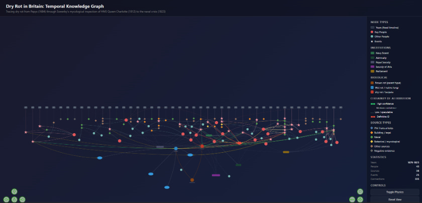
Dry Rot in Britain: Temporal Knowledge Graph — tracing the rot from Pepys (1684) through scientific classification to HMS Queen Charlotte (1812).
Every historian has a system for managing the chaos of the archive. Word documents, Excel spreadsheets, index cards, Zotero libraries, folders of hastily snapped photographs. The fundamental problem is always the same: as the material accumulates, the connections between sources begin to fray. You know you read something about a specific merchant six months ago, but where? You know two events in different colonies are related, but the evidence is scattered across three different files.
Historians have always been interested in relationships, the problem is that our note-taking systems have never matched that interest. A knowledge graph solves this by recording the links between entities as rigorously as the entities themselves. Instead of burying the connection in a flat sentence that says, “Kyd sent Banks information about myrobalans from Calcutta,” you create nodes (Kyd, Banks, myrobalans, Calcutta) and define the edges between them: sent to, located in, mentioned in. The note and the underlying structure become the exact same thing.
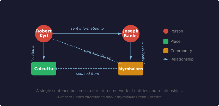
A single sentence, “Kyd sent Banks information about myrobalans from Calcutta,” becomes a structured network of entities and relationships.
If you’ve ever used Gephi or sketched a network diagram on a whiteboard, you already understand the concept. Nodes are entities: people, places, commodities, institutions, sources, events. Edges are the relationships binding them together.
The shift is simple but profound. In a Word document, information is organized chronologically by when you found it. In a spreadsheet, it is constrained by whatever columns you guessed you might need at the start. In a knowledge graph, information is organized by what it is actually about. Every new note automatically connects to everything you already know about those same people, places, and commodity chains.
I’ve been using this method to investigate when Serpula lacrymans, the destructive dry rot fungus, arrived in Britain. There is no bulk data to process here. This is entirely traditional research: searching through digitized eighteenth-century sources, following citation trails, cross-referencing dates. The kind of work where you are deep in Eighteenth Century Collections Online and Google Books, chasing footnotes between building manuals, parliamentary records, botanical surveys, and newspaper archives.
Now, every time I find a new source, I don’t add a line to a spreadsheet. I add nodes and edges. The graph has 43 people, 62 sources, 25 events, 2 organisms, 60 relationships, and 15 open questions, all in a single JSON file. Claude Code handles the data entry. I describe what I’ve found in plain English, and it maintains the structured knowledge graph and an interactive timeline visualization.
The graph forces distinctions that flat notes let you fudge. Samuel Pepys gathered toadstools “as big as my Fists” from neglected ship holds in 1684, and that’s often cited as early evidence of dry rot. But when I added Pepys as a source node and connected it to the organism nodes, the graph forced a question: which organism? The conditions Pepys describes are textbook for native wet rot, not the invasive Serpula. Because the graph holds both organisms as separate nodes with distinct diagnostic features, that distinction stays visible every time a new source mentions “rot.”
The graph also holds what I don’t know. Those 15 open question nodes (missing volumes, unverified claims, sources I haven’t yet read) are as important as the evidence nodes. In a Word document, unanswered questions get buried between paragraphs. In a graph, they stay visible, connected to the sources that raised them, waiting.
The dry rot graph is small and growing, but the Joseph Banks leather project demonstrates what happens when this method scales up and merges with machine transcription.
It started with a trip to the Sutro Library in San Francisco, where I photographed 181 handwritten letters related to the British leather trade (1797–1817). I used Claude Code to write processing scripts, which sent the photographs to Google’s Gemini for handwriting recognition, extracted structured entities from the transcriptions, and output the results as nodes and edges. I then read the key letters in chronological order to confirm the Gemini transcriptions and better understand the knowledge transmission between India and London.
I then integrated the full correspondence network from Warren Dawson’s Calendar of the Banks Letters, nearly 7,000 entries, and pulled in select figures related to leather and India from Neil Chambers’ Indian and Pacific Correspondence. But the core of the work was still note-taking. I was trying to answer a specific question: How did Banks identify catechu as a viable tanning agent?
The resulting leather network contains 275 people, 55 commodities, 119 places, and 46 institutions (495 nodes and 1,191 connections). That is a modest dataset, but it revealed global connections that sequential reading simply couldn’t.
The graph made it visually apparent that Banks operated as a switchboard connecting Indian botanical research directly to British industrial policy, routing knowledge between people who would never otherwise have crossed paths. Robert Kyd at the Calcutta Botanic Garden, Charles Jenkinson in the House of Lords, Samuel Purkis the tanner, and Andrew Berry conducting tanning experiments. The graph reveals them as vital components of a single coordinated commodity network, with Banks at the center.
Working through the graph drove new biographical research. It surfaced surprises, like the fact that Samuel Purkis and Humphry Davy were friends before Davy began working with Banks, and that Purkis had been corresponding with Banks throughout the 1790s. The graph didn’t explain the connection, but it surfaced it, turning a static name on a letter into a vibrant research question.
Anyone who has attended a digital humanities conference knows the problem with network graphs: they often look like impenetrable hairballs. Generated by NetworkX or Gephi with default settings, they are technically correct but analytically useless. You can’t tell what the graph is arguing because the layout isn’t designed to argue anything, it’s just a physics simulation.
Claude Code built the visualizations for the leather project too, and the one I’m most excited about is a temporal network.
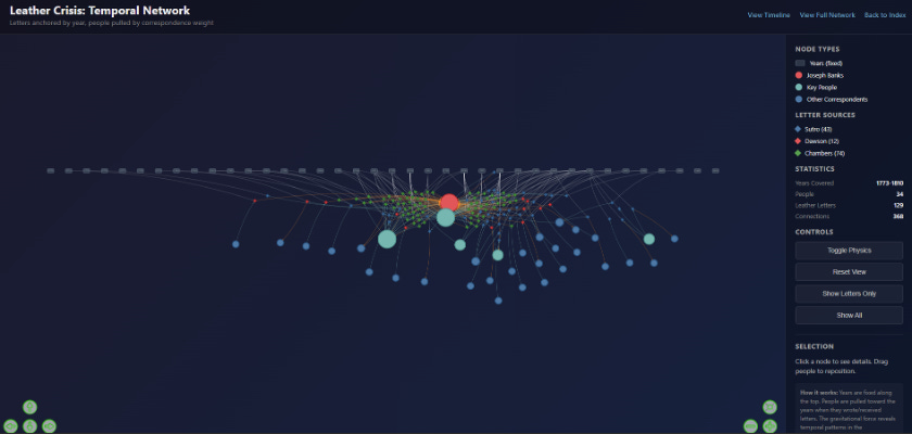
Leather Crisis: Temporal Network, years anchored along the top, people pulled by correspondence weight.
Standard tools force you to choose between a timeline or a network graph. The temporal network fuses them. Years are fixed along the x-axis, and people float below, gravitationally pulled toward the years when they were most active. You can actually watch the network grow as the tanning crisis develops, spotting the transition as the conversation shifts from botanical science to industrial policy. This hybrid layout didn’t exist in a dropdown menu. It emerged from describing what I wanted to see and letting the AI implement it.
Because Claude Code builds through natural conversation, each visualization matches the specific historical question. Before this, custom visualizations were simply out of reach for most historians; you either used what Gephi, QGIS or Tableau offered or you didn’t visualize at all. Now, iterative, question-driven visualization is just another part of the research workflow.
The dry rot and leather graphs are personal research tools: my nodes, my edges, my questions. But this exact logic scales up to major linked open data projects.
Take LINCS (Linked Infrastructure for Networked Cultural Scholarship), a project building linked open data infrastructure for cultural heritage in Canada. Our Historical Canadians dataset builds on the Dictionary of Canadian Biography with Wikidata, modeling familial connections, occupations, and residences using CIDOC-CRM, all queryable via SPARQL.
That is the far end of the spectrum: formal ontologies, institutional infrastructure, and strict interoperability. My personal graphs are not FAIR data (not Findable, Accessible, Interoperable, or Reusable in the formal sense). I can and do share them, but they are not interoperable. Making them so would mean modeling every entity against a formal ontology like CIDOC-CRM, reconciling every node to a persistent identifier, and minting URIs when the PIDs do not exist, a significant step up from a JSON file and a conversation with Claude. The underlying logic, entities and relationships, is the same, but the distance between a personal research graph and a LOD dataset is real.
That said, we are actively experimenting with using LLMs to reduce this barrier, and the results are promising. But today, there is no easy path from a Claude subscription to standards-compliant linked data. The habits of structured thinking you develop when building a small graph are exactly the habits required to engage with large-scale projects like LINCS, but the tooling to bridge that gap is still emerging.
The barrier to entry has collapsed. You don’t need a massive grant or a dedicated developer to start. You just need a compelling historical question, a willingness to think in nodes and edges, and the right AI tools to help you build. If you’re a historian still managing the chaos of the archive in Word documents and spreadsheets, consider nodes and edges instead. Start small. The graph will grow with your research, and you might be surprised by the connections it reveals.
Enjoy the article? Share with one friend, or even better, your socials.