Introduction to the precision-recall plot

The precision-recall plot is a model-wide measure for evaluating binary classifiers, closely related to the ROC plot but more informative when the dataset is imbalanced. This page covers the basic concept and several important aspects of the plot.

Key points

The precision-recall plot puts recall on the x-axis and precision on the y-axis. Recall is the same measure as sensitivity.
Precision is calculated from the predicted positives, not from one observed class, so it is the only one of these measures that responds to the ratio of positives and negatives.
The baseline is not a diagonal. A random classifier gives the horizontal line P / (P + N), so the baseline drops as a dataset becomes more imbalanced.
Interpolation between two precision-recall points is non-linear, which is why many tools draw these curves inaccurately.
Every ROC point has a corresponding precision-recall point, so the two plots describe the same classifier while answering different questions.

For those who are not familiar with the basic measures derived from the confusion matrix or the basic concept of model-wide evaluation, we recommend reading the following two pages.

For those who are not familiar with the basic concept of the ROC plot, we also recommend reading the following page.

Introduction to the ROC (Receiver Operating Characteristics) plot

If you want to dive into making nice precision-recall plots right away, have a look at the tools page:

Tools for ROC and precision-recall

Precision-recall shows pairs of recall and precision values

The precision-recall plot is a model-wide evaluation measure that is based on two basic evaluation measures – recall and precision. Recall is a performance measure of the whole positive part of a dataset, whereas precision is a performance measure of positive predictions.

Four ovals respectively represent observed labels, four outcomes, recall, and precision. — A dataset has two labels (P and N), and a classifier separates the dataset into four outcomes – TP, TN, FP, FN. The precision-recall plot is based on two basic measures – recall and precision that are calculated from the four outcomes.

The precision-recall plot uses recall on the x-axis and precision on the y-axis. Recall is identical with sensitivity, and precision is identical with positive predictive value.

Why precision behaves differently from sensitivity and specificity

Recall is simply another name for sensitivity, so the precision-recall plot shares one of its two measures with the ROC plot. The other measure, precision, is calculated in a fundamentally different way, and that difference is the reason the precision-recall plot stays informative when a dataset is imbalanced.

Sensitivity and specificity are each calculated inside a single observed class. Sensitivity uses only the observed positives, and specificity uses only the observed negatives. Precision is calculated from the predicted positives instead, which combines counts taken from both observed classes.

Measure	Formula	Calculated from
Sensitivity (recall)	TP / (TP + FN)	observed positives only
Specificity	TN / (TN + FP)	observed negatives only
Precision	TP / (TP + FP)	predicted positives, drawn from both classes

This has a direct consequence. Neither sensitivity nor specificity changes when the number of negatives changes, because each stays within its own observed class. Precision has FP in its denominator, and the number of false positives grows as the number of negatives grows. Precision is therefore the only one of the three that responds to the ratio of positives and negatives.

The same classifier on a balanced and an imbalanced dataset

Let us assume a classifier with sensitivity 0.9 and specificity 0.9, applied to two datasets. The first is balanced, with 100 positives and 100 negatives. The second is imbalanced, with the same 100 positives but 10 000 negatives. The classifier behaves identically in both cases.

	Balanced (100 : 100)	Imbalanced (100 : 10 000)
TP	90	90
FN	10	10
FP	10	1000
TN	90	9000
Sensitivity	0.9	0.9
Specificity	0.9	0.9
Precision	90 / 100 = 0.9	90 / 1090 = 0.083

Sensitivity and specificity report 0.9 in both cases and give no hint that anything has changed. Precision falls from 0.9 to 0.083. The reason is visible in the denominator: the classifier now produces 1000 false positives against only 90 true positives, so fewer than 9 out of every 100 positive predictions are correct.

Nothing about the classifier changed between the two columns. Only the number of negatives did, and only precision noticed.

Precision answers the question a user of the model actually asks

The three measures answer three different questions.

Sensitivity: of all the actual positives, how many did the classifier find?
Specificity: of all the actual negatives, how many did it correctly reject?
Precision: of everything it predicted as positive, how much was right?

Only the third question is the one asked by someone who has to act on the predictions. If a genome-wide scan returns 1090 candidate genes and 1000 of them are wrong, the effort wasted on follow-up is governed by precision, not by sensitivity or specificity. This is what we mean by saying the precision-recall plot is more informative on imbalanced datasets: it reports the quantity that reflects what the model costs to use.

Plotting precision against the threshold value

For the same reason, some studies plot precision directly against the threshold value, or against the number of instances predicted as positive, rather than against recall. Such a plot answers the practical question of how reliable the positive predictions are at each operating point, which matters when only the top-ranked predictions will be examined in the laboratory. The precision-recall plot keeps the same information but presents it against recall, so that a single curve also shows how much of the positive class is being recovered.

A naïve way to calculate a precision-recall curve by connecting precision-recall points

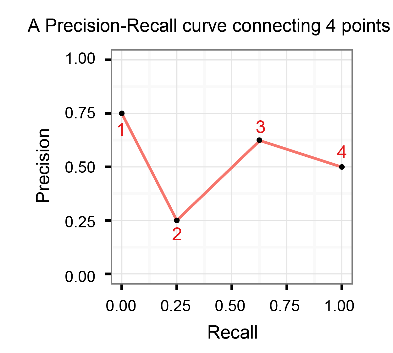
A precision-recall point is a point with a pair of x and y values in the precision-recall space where x is recall and y is precision. A precision-recall curve is created by connecting all precision-recall points of a classifier. Two adjacent precision-recall points can be connected by a straight line.

An example of making a precision-recall curve

We’ll show a simple example to make a precision-recall curve by connecting several precision-recall points. Let us assume that we have calculated recall and precision values from multiple confusion matrices for four different threshold values.

Threshold	Recall	Precision
1	0.0	0.75
2	0.25	0.25
3	0.625	0.625
4	1.0	0.5

We first added four points that matches with the pairs of recall and precision values and then connected the points to create a precision-recall curve.

A Precision-Recall curve and four Precision-Recall points. — The plot shows a precision-recall curve connecting four precision-recall points.

3 important aspects of making an accurate precision-recall curve

Unlike the ROC plot, it is less straight-forward to calculate accurate precision-recall curves since the following three aspects need to be considered.

Estimating the first point from the second point
- AUC cannot be calculated without the first point
Non-linear interpolation between two points
- curves with linear interpolation tend to be inaccurate for small datasets, imbalanced datasets, and datasets with many tied scores
Calculating the end point
- the end point should not be extended to the top right (1.0, 1.0) nor the bottom right (1.0, 0.0) except in the case that observed labels are either all positives or all negatives

We’ll show an example of these aspect by creating a precision-recall curve.

An example of recall and precision pairs

We use four pairs of recall and precision values that are calculated from four threshold values.

Point	Threshold	Recall	Precision
1	1	0	–
2	2	0.5	0.667
3	3	0.75	0.6
4	4	1	0.5

We explain the three aspects by using the three pairs of consecutive points.

Points 1-2: estimating the first point
Points 2-3: non-linear interpolation
Points 3-4: calculating the end point

Points 1-2: Estimating the first point from the second point

The first point should be estimated from the second point because the precision value is undefined when the number of positive predictions is 0. This undefined result is easily explained by the equation of precision as PREC = TP / (FP + TP) where (FP + TP) is the number of positive predictions.

There are two cases of estimating the first point depending on the true positives of the second point.

The number of true positives (TP) of the second point is 0
The number of true positives (TP) of the second point is not 0

Case 1: TP is 0

Since the second point is (0.0, 0.0) for this case, it is easy to estimate the first point, which is also (0.0, 0.0). In other words, the first point is not necessary to be estimated for this case.

Case 2: TP is not 0

This is also the case for our example, and the second point is (0.5, 0.667). We can estimate the first point by drawing a horizontal line from the second point to the y-axis. Hence, the first point is estimated as (0.0, 0.667).

First two Precision-Recall points. — Drawing a horizontal line from the second position to the y-axis to estimate the first point.

Points 2-3: Non-linear interpolation between two points

Davis and Goadrich proposed the non-linear interpolation method of precision-recall points in their article (Davis2006). The equation described in their article is

$\mathrm{y = \displaystyle \cfrac{TP_A + x}{TP_A + x + FP_A + \cfrac{FP_B - FP_A}{TP_B - TP_A} \cdot x}}$

where y is precision and x can be any value between 0 and |TP_B – TP_A|. Smooth curves can be created by calculating many intermediate points between two points A and B.

Non-linear interpolation of two Precision-Recall plots. — Two precision-recall points are connected non-linearly. The blue dot line shows a straight line between points 2 and 3, whereas the red solid curve shows the correct non-linear interpolation between them.

An intermediate point 2.5 for points 2-3

Let us assume the second point has 2 TPs and 1 FP and the third point has 3 TPs and 2 FPs.

Point 2: (0.5, 0.667)
Point 3: (0.75, 0.6)

	Point 2	Point 3
TP (# of true positives)	2	3
FP (# of false positives)	1	2
Recall	0.5	0.75
Precision	0.667	0.6

We then define the intermediate point 2.5 as the middle point where recall is 0.625. We show that the precision value of point 2.5 can be different for linear and non-linear interpolation.

Linear interpolation

Since point 2.5 is the center point of the second and the third points, the precision value is 0.633.

Point 2.5: (0.625, 0.633)

Non-linear interpolation

We calculate the precision value by

$\mathrm{\displaystyle \cfrac{TP_{point2} + x}{TP_{point2} + x + FP_{point2} + \cfrac{FP_{point3} - FP_{point2}}{TP_{point3} - TP_{point2}} \cdot x}}$

with the following values.

TP_point2: 2
FP_point2: 1
TP_point3: 3
FP_point3: 2
x: 0.5

The calculated precision value is 0.625.

Point 2.5: (0.625, 0.625)

Points 3-4: Calculating the end point

The end point of the precision-recall curve is always (1.0, P / (P + N)), since recall reaches 1.0 once every instance is predicted as positive. For instance, the end point is (1.0, 0.5) from (1.0, 4 / (4 + 4)) when P is 4, and N is 4. Subsequently, the end position and the previous position should be connected by non-linear interpolation.

The end point of a Precision-Recall curve. — The precision value at the end point can be calculated as P / (P + N). It is 0.5 when P is 4 and N is 4.

Interpretation of precision-recall curves

Similar to a ROC curve, it is easy to interpret a precision-recall curve. We use several examples to explain how to interpret precision-recall curves.

A precision-recall curve of a random classifier

A classifier with the random performance level shows a horizontal line as P / (P + N). This line separates the precision-recall space into two areas. The separated area above the line is the area of good performance levels. The other area below the line is the area of poor performance.

Two Precision-Recall curves of random classifiers for different positive and negative ratio. — A random classifier shows a straight line as P / (P + N). For instance, the line is y = 0.5 when the ratio of positives and negatives is 1:1, whereas 0.25 when the ratio is 1:3.

A precision-recall curve of a perfect classifier

A classifier with the perfect performance level shows a combination of two straight lines – from the top left corner (0.0, 1.0) to the top right corner (1.0, 1.0) and further down to the end point (1.0, P / (P + N)).

Two Precision-Recall curves of perfect classifiers for different positive and negative ratio. — A perfect classifier shows a combination of two straight lines. The end point depends on the ratio of positives and negatives. For instance, the end point is (1.0, 0.5) when the ratio of positives and negatives is 1:1, whereas (1.0, 0.25) when the ratio is 1:3.

Precision-recall curves for multiple models

It is easy to compare several classifiers in the precision-recall plot. Curves closer to the perfect precision-recall curve have a better performance level than those closer to the baseline. In other words, a curve above the other curve has a better performance level.

Two Precision-Recall curves for two classifiers A and B - The plot indicates classifier A outperforms classifier B. — Two precision-recall curves represent the performance levels of two classifiers A and B. Classifier A clearly outperforms classifier B in this example.

Noisy curves for small recall values

A precision-recall curve can be noisy (a zigzag curve frequently going up and down) for small recall values. Therefore, precision-recall curves tend to cross each other much more frequently than ROC curves especially for small recall values. Comparisons with multiple classifiers can be difficult if the curves are too noisy.

AUC (Area Under the precision-recall Curve) score

Similar to ROC curves, the AUC (the area under the precision-recall curve) score can be used as a single performance measure for precision-recall curves. As the name indicates, it is an area under the curve calculated in the precision-recall space. An approximate but easy way to calculate the AUC score is using the trapezoidal rule, which is adding up all trapezoids under the curve.

The AUC score can be calculated by the trapezoidal rule. — The areas of the three trapezoids 1, 2, 3 are 0.335, 0.15875, and 0.1375. The AUC score is then 0.63125.

Although the theoretical range of AUC score is between 0 and 1, the actual scores of meaningful classifiers are greater than P / (P + N), which is the AUC score of a random classifier.

Four Precision-Recall curves with their AUC scores. — The score is 1.0 for the classifier with the perfect performance level (P) and 0.5 for the classifier with the random performance level (R). The plot clearly shows classifier A outperforms classifier B, which is also supported by their AUC scores (0.7 and 0.52).

One-to-one relationship between ROC and precision-recall points

Davis and Goadrich introduced the one-to-one relationship between ROC and precision-recall points in their article (Davis2006). In principle, one point in the ROC space always has a corresponding point in the precision-recall space, and vice versa. This relationship is also closely related to the non-linear interpolation of two precision-recall points.

A ROC curve and a precision-recall curve should indicate the same performance level for a classifier. Nevertheless, they usually appear to be different, and even interpretation can be different.

In addition, the AUC scores are different between ROC and precision-recall for the same classifier.

Difference of the AUC scores between ROC and Precision-Recall. — ROC shows the same AUC score for A (0.61) and B (0.61), but precision-recall shows different scores for A (0.62) and B (0.53).

3 important characteristics of the precision-recall plot

Among several known characteristics of the precision-recall plot, three of them are important to consider for accurate precision-recall analysis.

Interpolation between two precision-recall points is non-linear.
The ratio of positives and negatives defines the baseline.
A ROC point and a precision-recall point always have a one-to-one relationship.

These characteristics are also important when the plot is applied to imbalanced datasets. For more details about the precision-recall plot with imbalanced datasets, we recommend reading the following pages.

How to cite

If this page has been useful in your work, please cite our article.

[Saito2015] Takaya Saito and Marc Rehmsmeier (2015) The precision-recall plot is more informative than the ROC plot when evaluating binary classifiers on imbalanced datasets. PLoS One. 10(3):e0118432. doi:10.1371/journal.pone.0118432

Ready-to-paste BibTeX and RIS entries are on our References page.