RL Scaling Laws for LLMs

Scaling is one of the most impactful concepts in the history of AI research. For large language models (LLMs), scaling has mostly been studied in the context of pretraining, where rigorous scaling laws have allowed us to clearly define the relationship between compute and performance. Inspired by these predictable trends, the LLM research community has empirically validated pretraining scaling laws across several orders of magnitude. Through this process, we have discovered that meaningful improvements in model capabilities can be consistently achieved by investing more data and compute into pretraining.

“The way ML used to work is that people would just tinker with stuff and try to get interesting results. That’s what’s been going on in the past. Then the scaling insight arrived. Scaling laws, GPT-3, and suddenly everyone realized we should scale. This is an example of how language affects thought. Scaling is just one word, but it’s such a powerful word because it informs people what to do.” - Ilya Sutskever

The success of scaling laws in the context of pretraining has inspired the same concept of scaling to be applied in other areas of the LLM training process. Most notably, scaling now plays a key role in reinforcement learning (RL), where researchers have demonstrated smooth and predictable model capability improvements with larger-scale training. In this overview, we will study scaling laws in the context of RL. Rather than studying this topic in isolation, however, we will first build a deep understanding of scaling laws for pretraining and aim to outline how scaling laws have evolved in their application to RL. As we will see, the exact definition of scaling laws is completely different between these two domains, but the fundamental concept of scale remains powerful in both.

Many early advancements in LLMs were driven by scaling up the pretraining process. Put simply, investing more compute into pretraining—by training a larger model on more data—yields better performance. We can rigorously define the relationship between compute and performance via a scaling law [13], or an equation that models the decrease in an LLM’s test loss as compute increases. As we will see, the pretraining process for an LLM follows smooth trends that can be accurately predicted via a scaling law, allowing the performance of larger models to be estimated before they are even trained. This ability to granularly forecast the expected result of a certain training configuration has many benefits:

• Significant compute investments are less daunting, as we know what the result of this invested compute will be.

• Iteration speed for experiments can be increased by running smaller scale experiments and extrapolating their results.

We will now build an understanding of scaling laws for LLM pretraining from the ground up. This knowledge of the mechanics and practical application of scaling laws for pretraining is needed to form a contrast with the scaling laws used for RL training. Pretraining scaling laws are highly standardized and follow a well-defined approach to estimate very particular training metrics. On the other hand, RL scaling laws—while still informative—tend to be much messier and bespoke, both in terms of their structure and the quantities that we measure.

Further learning. Although we cover the key details of pretraining scaling laws in this section, this is a popular and complex topic with a long history of study. For more details and links to further reading, please see the overview above.

We can model the LLM pretraining process with a power law. At the simplest level, a power law describes a relationship between two quantities. A basic power law can be expressed as y = a × x^p. The two quantities being studied are x and y, while a and p are constants that describe their relationship—a controls the vertical position of the curve, while p controls the steepness or direction of the curve. Plotting this simple power law function gives us the figure shown below.

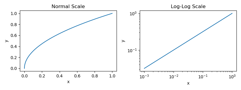
We provide the power law plot in both normal and log scale because most papers that study LLM scaling laws tend to plot their results in log scale. However, the plots provided for LLM scaling do not look like the plot shown above—they are usually flipped upside down; see below for an example. This is just an inverse power law, which can be formulated as y = a × (1 / x)^p. This is nearly identical to a standard power law, but we just use a negative exponent for p. As we can see below, using a negative exponent for p flips the power law plot upside down.

LLM power laws. This inverse power law, when plotted with a log scale, yields the signature linear relationship that characterizes LLM scaling laws. The two quantities we model via this inverse power law in LLM pretraining are:

1. The LLM’s test loss L—the next token prediction or cross entropy loss in particular (or another entropy-based metric like bits-per-byte or perplexity)—measured over an in-distribution, held-out validation set.

2. The compute C spent during pretraining that is estimated via the number of training FLOPs C = 6 × N × D, where N is the number of model parameters and D is the number of tokens observed during pretraining.

The factor of six used when estimating training compute comes from the fact that the LLM performs a single forward and backward pass during each training step. A single forward pass costs about 2N FLOPs per token, and the backward pass is 2× the cost of the forward pass. Therefore, a training step costs about 6N FLOPs per token, and we multiply this quantity by the total number of tokens observed during training to yield the C = 6 × N × D approximation. This approximation of pretraining compute was used in one of the first papers to study pretraining scaling laws [13], leading to its adoption in other work on the topic.

To develop a more concrete understanding of scaling laws for pretraining, we will overview two seminal papers [13, 14] that established the foundational principles of scaling. In [13], authors study the impact of several settings on the pretraining process, discovering that performance improves smoothly as we increase:

1. Model parameters.

2. Data volume.

3. Training compute.

More specifically, a power law relationship is observed between each of these factors and the LLM’s test loss when performance is not bottlenecked by either of the other two factors. To observe these power laws, LLMs with sizes up to 1.5B parameters are trained on several subsets of the WebText2 corpus. As shown below, the performance of these models steadily improves as we increase model size, data volume, or compute. These trends span eight orders of magnitude in compute, six orders of magnitude in model size, and two orders of magnitude in dataset size. The exact power law relationships and equations are provided below.

Each of these equations is very similar to the inverse power law equation that we saw before, but we set a = 1 and have an additional multiplicative constant (i.e., C_c, D_c, or N_c) inside of the parenthesis. To fit these power laws, we train a collection of models with different sizes while varying the amount of compute and data used for training. We can then measure the test loss for each of these models, forming a dataset of training configurations with a corresponding test loss. We can then fit the parameters of our power law to this data. Although there are many ways to fit a power law, one common approach for simple power law relationships is to fit a linear model on the observed data in log-log space.

What do power laws tell us? Although the power law plots provided above look promising, we should notice that these plots are generated using a log scale. If we generate normal plots (i.e., without log scale), we get the figures below, where we see that the shape of the power law resembles an exponential decay. In this way, increasing the quality of an LLM becomes exponentially more difficult with scale.

Compute-optimal allocation. The key scaling trends for LLM pretraining were established in [13], where we see that the LLM’s test loss follows smooth power law trends with compute, model parameters, and data volume. One important takeaway from this analysis is that, given a fixed compute budget, we get the best results by training a larger model over less data—usually ending the training process before the model fully converges. Chinchilla [14] builds upon this analysis with an extensive study of optimal compute allocations for pretraining. In particular, the analysis in [14] studies how to optimally allocate a fixed compute budget between model parameters and the number of training tokens to minimize the test loss.

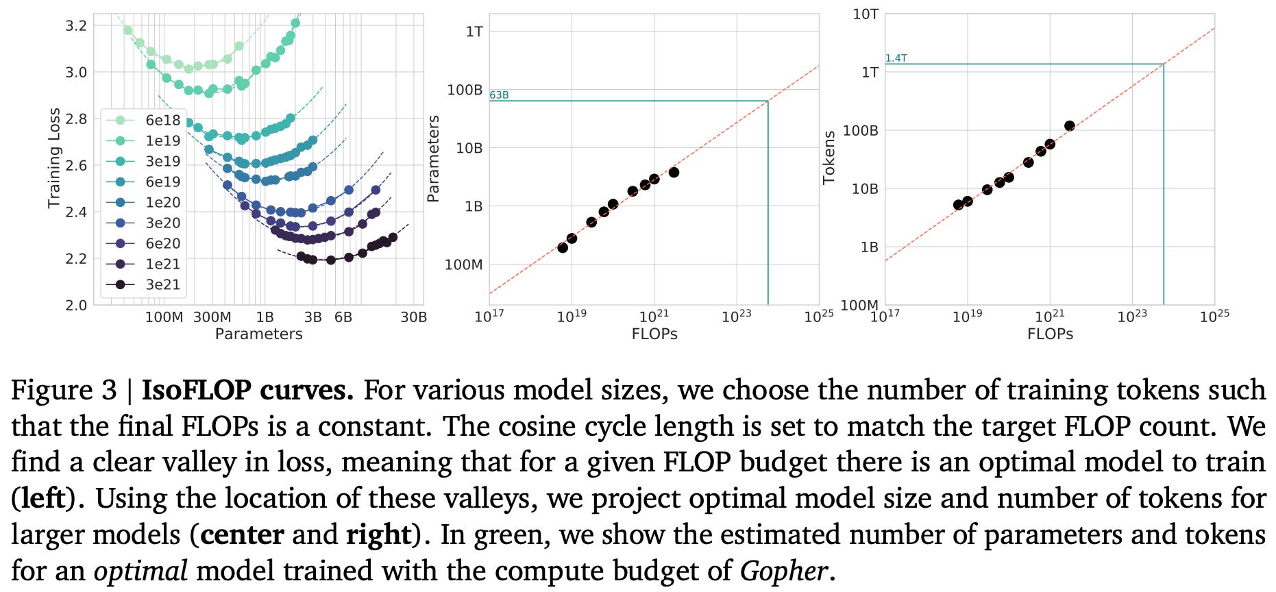
By training over 400 LLMs of varying sizes over different amounts of data, we learn that the scaling recommendations provided in [13] lead most LLMs to be undertrained—training these models on more data would yield better results. More specifically, Chinchilla finds that model and data scale should be increased proportionally for pretraining to be compute optimal; see above. This study is conducted using the same scaling law formulations, but authors explicitly sweep various model and data size combinations under a fixed compute budget to find the optimal balance of data and parameters for minimizing test loss.

Until recently, most of the compute used for training an LLM was invested into pretraining. We mostly focused on scaling up the pretraining process, while post-training was a less expensive endeavor used to optimize a model’s style and behavior. The advent of reasoning models drastically changed these standards.

“Scaling RL compute is emerging as a critical paradigm for advancing LLMs. While pre-training establishes the foundations of a model; the subsequent phase of RL training unlocks many of today’s most important LLM capabilities, from test-time thinking to agentic capabilities… Deepseek-R1-Zero used 100,000 H800 GPU hours for RL training – 3.75% of its pre-training compute. This dramatic increase in RL compute is amplified across frontier LLM generations, with more than 10× increase from o1 to o3 and a similar leap from Grok-3 to Grok-4.” - from [1]

Compared to a standard LLM, reasoning models output a long reasoning trace or chain of thought—typically encapsulated by <think> … </think> tokens—before providing a final answer. This idea was popularized by OpenAI’s o-series models, which demonstrated drastic improvements in reasoning capabilities by training models to generate reasoning tokens prior to their final answer. The initial release of o1 highlighted two important new axes of scaling:

1. RL training compute.

2. Inference-time compute.

As shown in the figure below, we observe a smooth increase in performance—resembling a scaling law—by increasing RL training and inference-time compute.

This breakthrough in reasoning was followed by the release of the open-weight DeepSeek-R1 [15] reasoning model, which performed on par with o1 and provided a technical report describing how the model was trained. Today, such reasoning capabilities have become the new standard for both open and closed models.

RL for reasoning. Reasoning models are trained via RL with verifiable rewards. As shown above, model performance improves as we scale up the RL training process. As a result, recent LLM research has heavily focused on scaling RL training for verifiable tasks (e.g., math or coding). Large-scale RL training has unlocked huge improvements in general reasoning capabilities and the quality of coding agents. However, a non-negligible fraction of total training compute is now being spent on RL, and optimally allocating compute for RL is difficult.

For pretraining, we use known scaling laws to reason about how to properly invest available compute—these laws provide a standardized understanding of how performance changes with model size, data, and compute. Given that compute is the primary bottleneck to AI progress, we need analogous scaling laws that enable us to better understand and predict the results of RL training at scale.

We will soon build upon our understanding of pretraining scaling laws to study RL scaling laws. However, we cannot properly interpret the scaling properties of RL without first understanding the basics of the RL training process. In this section, we will briefly outline the key concepts needed for this discussion, focusing on the GRPO algorithm and its many variants. We focus on GRPO in particular because it is the most common algorithm to use for large-scale RL training with reasoning models—at least in publicly disclosed research. For example, the popular DeepSeek-R1 reasoning model [15] uses GRPO for RL training.

“We introduce the Group Relative Policy Optimization (GRPO), a variant of Proximal Policy Optimization (PPO). GRPO foregoes the critic model, instead estimating the baseline from group scores, significantly reducing training resources.” - from [4]

Proposed in [4], GRPO is an RL optimization algorithm that builds upon prior algorithms like Proximal Policy Optimization (PPO). Whereas PPO was the most popular RL optimizer for LLMs in the RLHF era, GRPO is now almost universally used for large-scale RL with reasoning models1. GRPO is a simpler and lighter weight optimizer compared to PPO, which has aided its adoption by the LLM research community (especially for open research). The main change made by GRPO relative to PPO is in the advantage estimation technique.

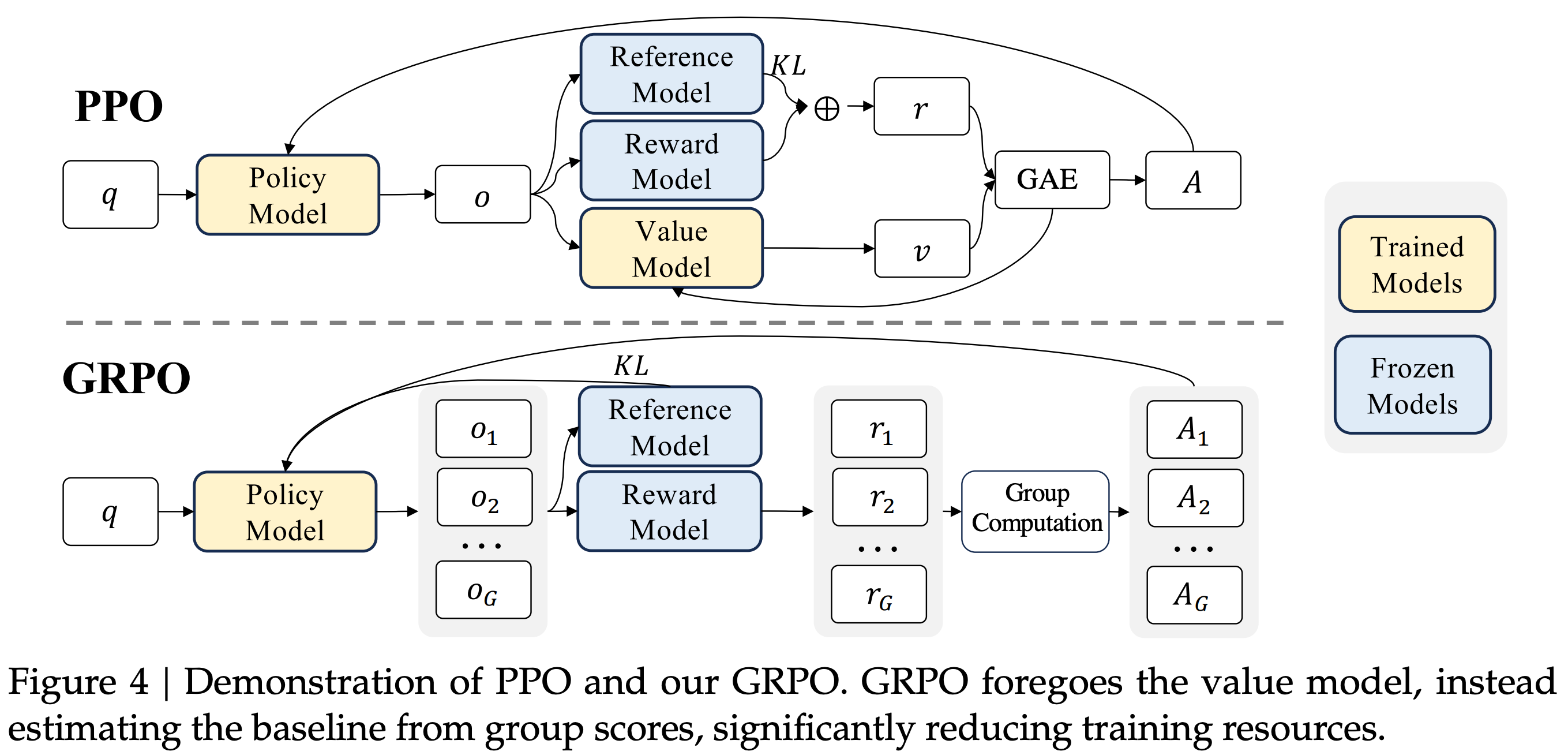
Instead of using a value model and GAE to estimate advantage as in PPO, GRPO estimates the advantage by sampling multiple completions or rollouts (i.e., a “group” of completions) for each prompt in a batch and using their rewards to form a baseline. This group-derived baseline replaces the value function and allows GRPO to not train a value model, thus drastically reducing the memory and compute overhead of RL training. Concretely, the advantage for completion i is computed by normalizing the reward for this completion r_i with the mean and standard deviation of rewards in the group; see below. The same advantage value is assigned to every token t in the completion.

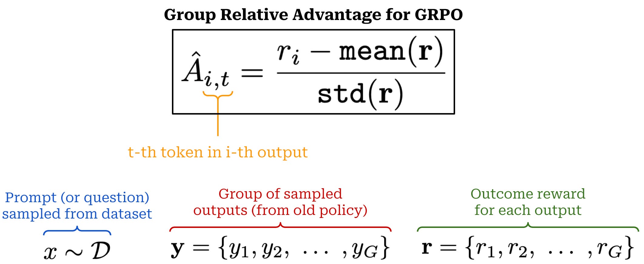
Intuitively, GRPO looks at the relative difference in rewards between multiple completions to the same prompt. The advantage is defined as the delta of one completion’s reward relative to the average reward observed in a group. This approach teaches the model to emphasize completions with higher-than-average reward.

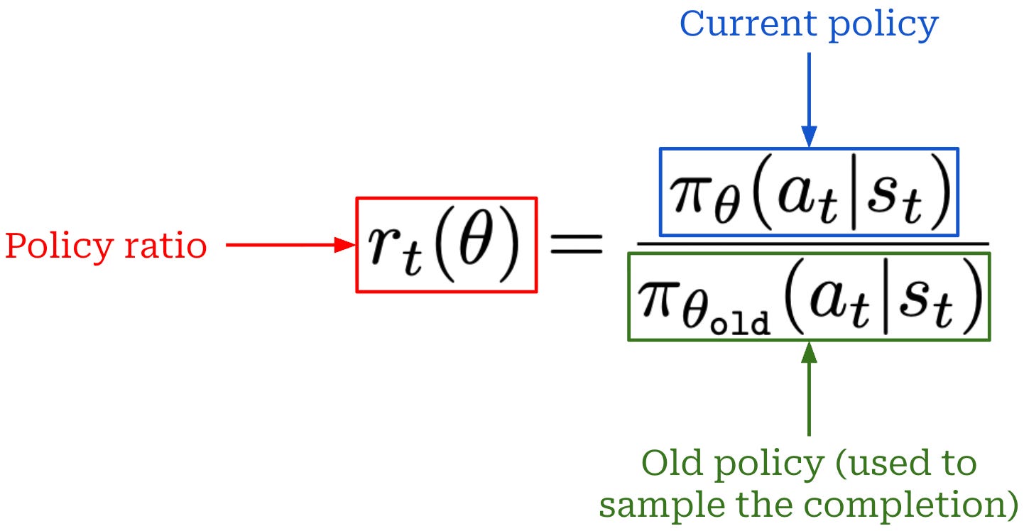
Loss function. Once the advantage has been computed, the loss function used for GRPO is quite similar to that of PPO. The center point of the loss function for both PPO and GRPO is the token-level policy (or importance) ratio. Specifically, this is the ratio of the probability assigned to a token by the current policy and the policy used to generate the rollout (i.e., the “old” policy); see below.

Using this policy ratio and the advantage, we can compute the loss function for GRPO as shown below. This loss function uses the same clipping mechanism proposed by PPO; see here for more details. Similarly to PPO, GRPO takes the minimum of a clipped and unclipped objective in its loss formulation, where the objective is just the product of the policy ratio and advantage for token t.

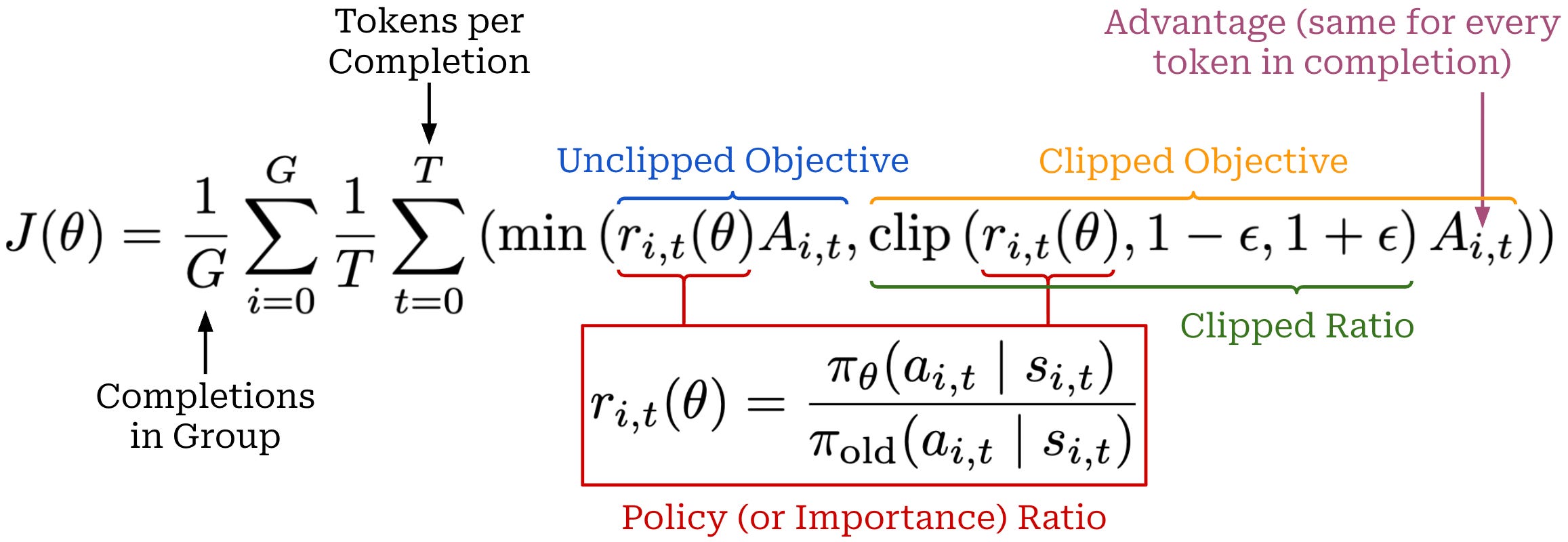
The inner term of the loss function for GRPO is computed on the token level. By default, we aggregate this loss over our batch by:

1. Averaging the token-level losses within each completion.

2. Averaging completion-level losses over the group.

The exact manner in which we aggregate the loss in GRPO can change, and we will soon see that the manner in which we aggregate loss over a batch can impact performance. Given that GRPO computes advantage based on group-level reward statistics, we must sample a large number of completions per prompt to obtain a reliable advantage estimate. As a result, GRPO usually needs relatively large batch sizes in order for training to be stable2; see here for more details.

GRPO & reward models. GRPO is mostly used in verifiable reward settings without a neural reward model. A common misconception about GRPO is that it eliminates the need for a reward model, but GRPO can be used with or without a reward model. In fact, the original GRPO paper [4] used a reward model instead of verifiable rewards! Removing the reward model is a benefit of verifiable rewards, not an intrinsic benefit of GRPO itself—the primary advantage of GRPO is the elimination of the value model. For more details on GRPO, including example code and a discussion of prior work that led to GRPO, please see the overview below.

The GRPO algorithm exploded in popularity after the release of DeepSeek-R1 [15] as many researchers began to replicate or extend results from the paper. Despite details of the model being openly published, fully replicating the training pipeline for DeepSeek-R1 proved non-trivial, leading many subsequent works to propose tweaks to the GRPO algorithm. In this section, we will overview the most successful modifications that are now commonly adopted for better RL training.

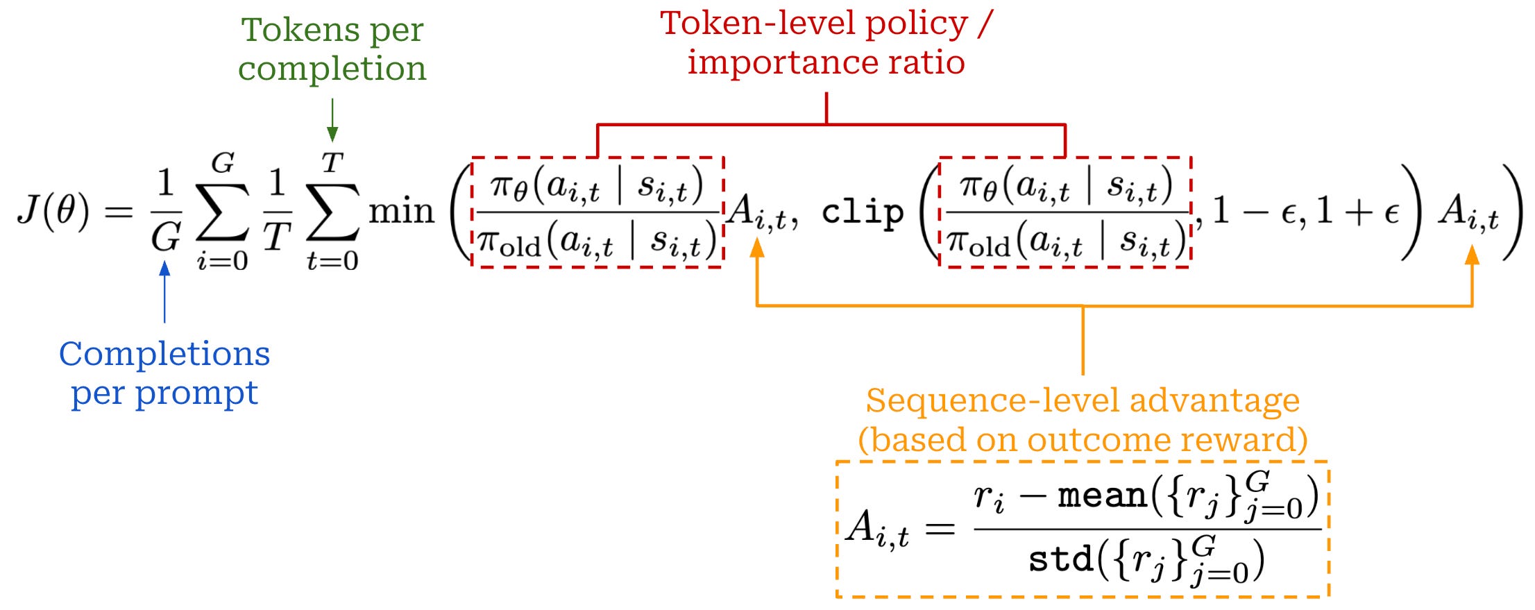
Group Sequence Policy Optimization (GSPO) [5] modifies the GRPO objective by computing the policy ratio on a sequence level rather than at the token level. The GRPO loss (shown above) introduces a misalignment between how the model is optimized and how rewards (or advantages) are assigned:

• Advantage is computed at the sequence level (in an outcome reward setting).

• Policy ratios—and the loss in general—are computed at the token level.

As shown in [5], per-token policy ratios tend to have high variance during RL training, which increases the variance of policy gradients and, in turn, leads to training instability. Specifically, the high variance of policy ratios can lead a single token to dominate the loss expression or even cause numerical instability during the RL training process. This problem is particularly acute when training LLMs on long sequences or using large, sparse Mixture-of-Experts models.

To protect against this variance, token-level importance ratios are clipped in the range [1 - ε, 1 + ε]. This clipping operation is formulated such that tokens have zero contribution to the gradient update if they are clipped within the objective. The importance ratio captures the change in a token’s probability after multiple policy updates over the same data—we clip tokens for which we observe a sufficiently large change in their probability. However, simply removing the contribution of these tokens to the policy gradient can be problematic. These can be rare (low probability) tokens that are identified as important by the policy update. Such tokens may capture key reasoning steps that the model needs to learn, but we suppress the learning process via the clipping operation.

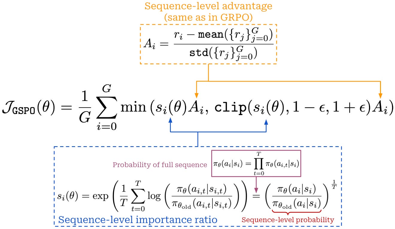
The key idea of GSPO is to compute importance ratios for the sequence rather than each token. Once we have derived the sequence-level importance ratio, the GSPO training objective is almost identical to that of GRPO; see above. We apply clipping to the sequence-level importance ratio, use the same advantage, and take a minimum of clipped and unclipped objectives at the sequence level.

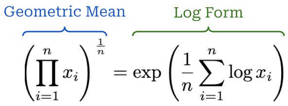
The sequence-level importance ratio can be derived by factorizing the probability of a sequence into a product of individual token probabilities. However, authors in [5] choose to define the sequence-level importance ratio using the logarithmic form of a geometric mean, which is defined as shown below. This geometric mean is taken over token-level probabilities, which normalizes the sequence-level policy ratio by the length of the sequence. By using this approach, we ensure that importance ratios for sequences of different lengths are comparable, as well as improve numerical stability—especially for long sequences—by formulating the ratio as a sum over logprobs instead of a product over raw probabilities.

We see in [5] that GSPO improves training stability, sample efficiency, and overall performance. The stability of GSPO is found to be especially useful when training large MoE models, such as Qwen3-235B-A22B. For these reasons, GSPO was adopted in the training process for the popular Qwen 3 model series.

Dynamic Sampling Policy Optimization (DAPO) [6] is not a single algorithm, but rather a modified recipe that proposes several useful tweaks to the vanilla GRPO optimizer. We see in [6] that the vanilla GRPO optimizer suffers from notable issues like:

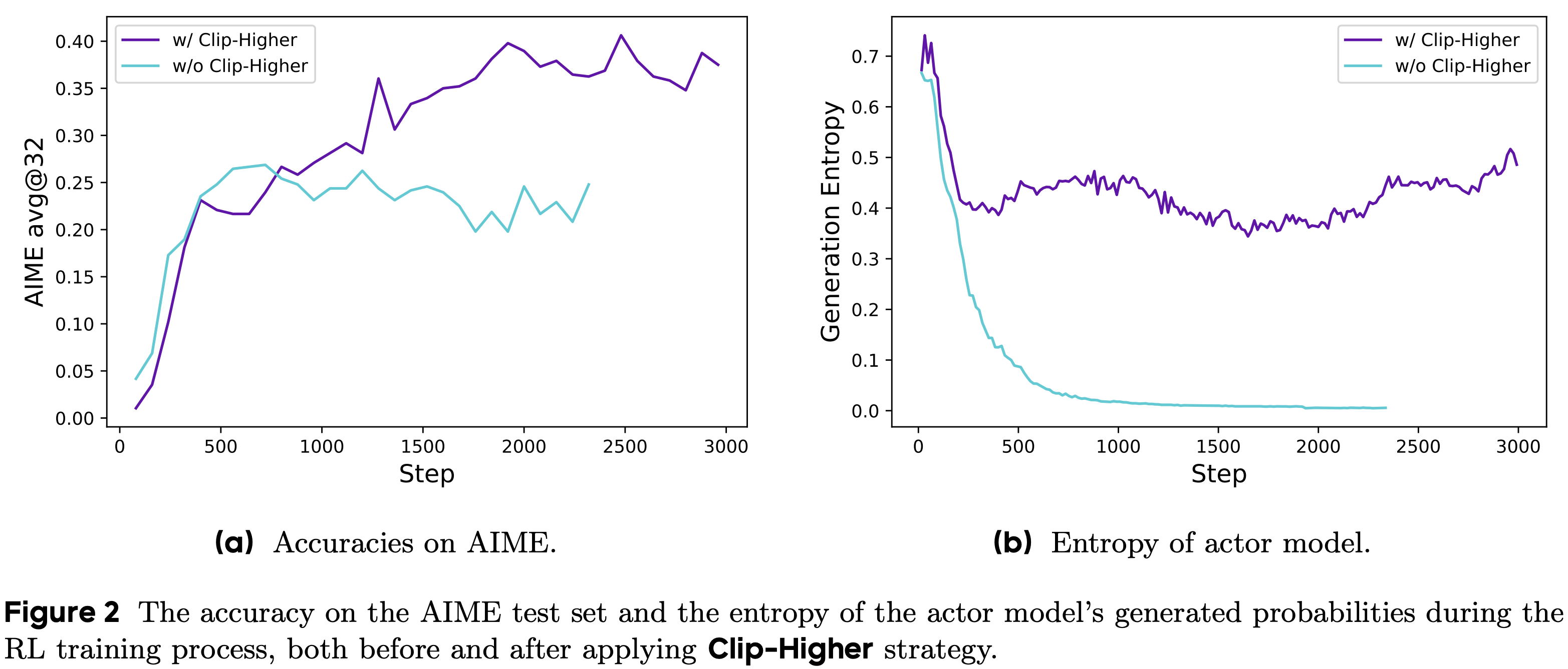
• Entropy collapse: the entropy of the model’s next token distribution collapses during the training process. Probability mass is primarily assigned to a single token and outputs are more deterministic.

• Reward noise: the training reward is very noisy and does not steadily increase during the RL training process.

• Training instability: the training process is unstable and may diverge.

To solve these issues, authors in [6] propose a suite of tricks that can be used in tandem. First, the entropy collapse problem in GRPO is shown to be caused by the fact that clipping emphasizes high probability tokens and punishes low probability (exploratory) tokens. The “clip higher” approach is proposed in [6] to solve this issue by decoupling lower and upper clipping bounds. Specifically, we clip in the range [1-ε_low, 1+ε_high], where ε_low=0.2 (default setting in GRPO) and ε_high=0.28 in [6]. Increasing ε_high prevents entropy collapse and improves overall GRPO performance; see below.

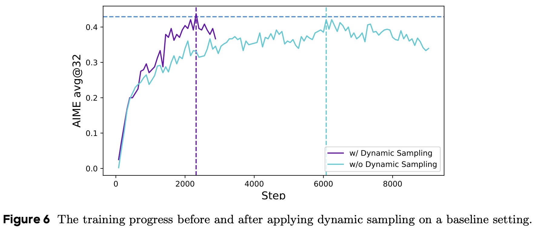
As RL training progresses, the number of samples for which all completions in a group are accurate increases. Such groups have zero advantage and, in turn, no impact on the policy gradient. As a result, these groups effectively reduce the batch size in GRPO, leading to noisier gradient estimates and degraded sample efficiency. Dynamic sampling is proposed in [6] to solve this problem by:

1. Filtering all prompts with perfect accuracy from a batch.

2. Continuing to sample prompts until we have a full batch.

This approach can increase the cost of constructing a batch, as we dynamically continue sampling prompts until the batch is full. However, we see in [6] that this cost is offset by the improved sample efficiency of RL training; see below.

Finally, DAPO also proposes a modified loss aggregation strategy and a new approach for handling completions that exceed the maximum sequence length. Vanilla GRPO aggregates token-level losses by i) computing the average loss in each sequence and ii) averaging sequence-level losses in the batch. However, this approach introduces a subtle bias—tokens within longer sequences have relatively less contribution to the overall batch gradient. To solve this, DAPO computes a token-level loss that is simply averaged over all tokens in the batch; see below.

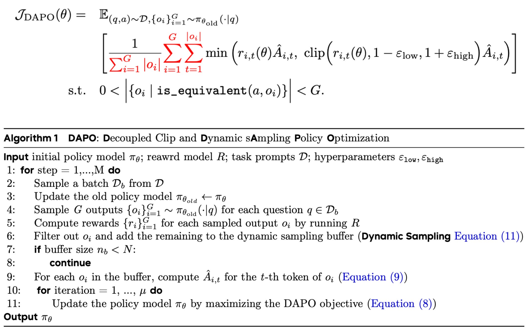
Additionally, a length-based penalty term is introduced to the reward to apply a “soft” punishment to completions that are too long. Instead of assigning a hard negative reward to any completion that exceeds the maximum sequence length, authors in [6] argue that we should slowly increase the overlong penalty to its maximum value as we approach the maximum sequence length. This approach provides a smooth length penalty from which the model can effectively learn.

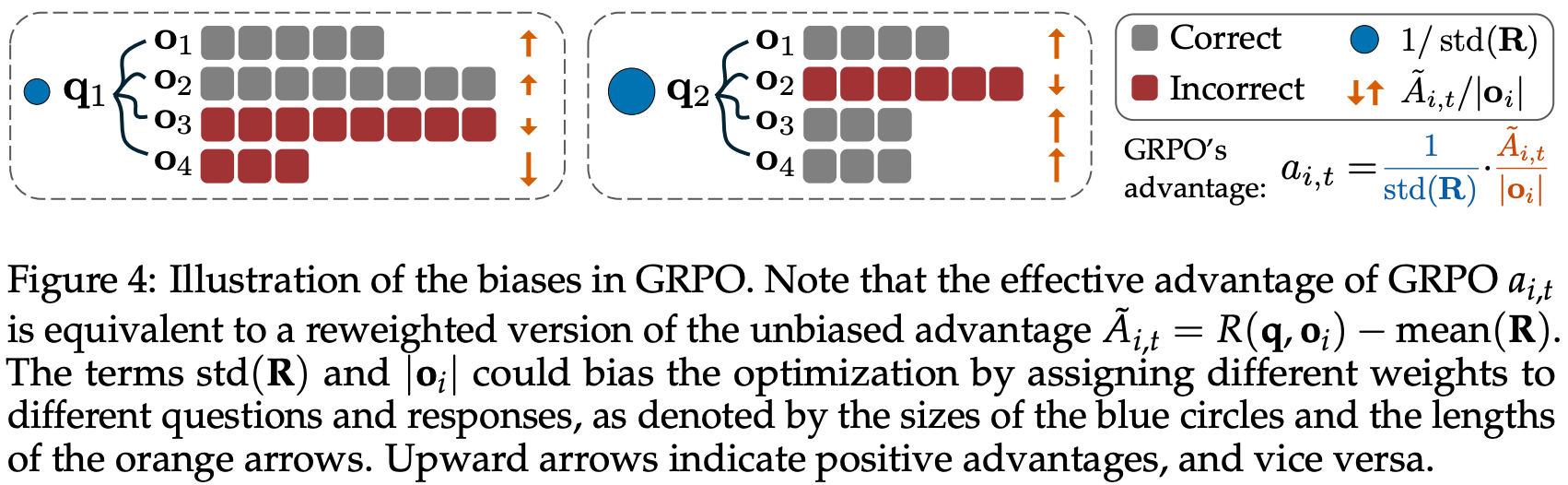
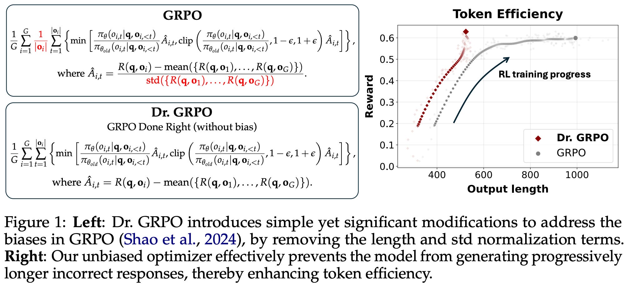
GRPO Done Right (Dr. GRPO) [7] outlined two key sources of bias that exist in the vanilla GRPO algorithm (depicted above):

1. Response-level length bias: GRPO normalizes the summed loss of tokens in each sequence by the total number of tokens in that sequence, leading to biased gradient updates based on the length of each response.

2. Question-level difficulty biases: the standard deviation term in the denominator of the advantage formulation in GRPO causes the advantage to become very large for questions that are either too easy (i.e., most responses have a reward of one) or too hard (i.e., most responses have a reward of zero).

To solve the first bias, Dr. GRPO aggregates the loss by summing token-level losses in a sequence and dividing this sum by a fixed constant MAX_TOKENS, thus removing response length from the aggregation process. The difference between this loss aggregation strategy and that of DAPO is nuanced. In DAPO, each token in the batch has an equal contribution to the gradient. As a result, DAPO still places more emphasis upon longer sequences in a batch, as these sequences have a larger ratio of total tokens (even if all tokens are weighted equally across the batch). On the other hand, replacing the sequence-level average with division by a fixed constant in Dr. GRPO effectively decouples aggregation from response lengths and, in turn, protects against length-based optimization bias.

The question-level difficulty bias is handled by removing the standard deviation term from the advantage estimator; see below. By making these two changes, Dr. GRPO improves training stability and efficiency, while making the resulting model more token efficient (i.e., responses are not artificially long).

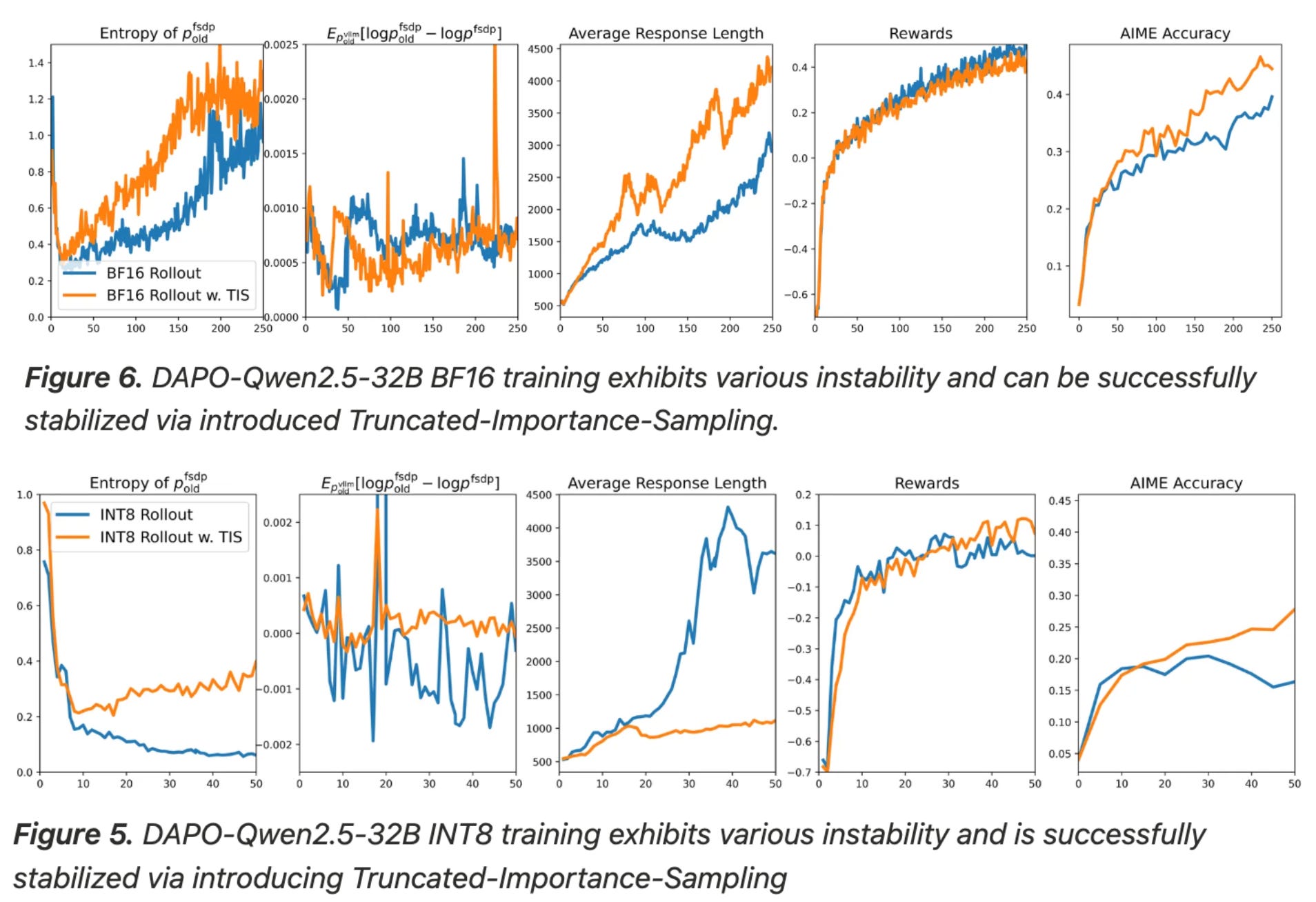
Truncated Importance Sampling (TIS) [9] attempts to address mismatches in token probabilities introduced by efficient RL training frameworks. As we know, there are two main operations that occur during RL training: i) sampling rollouts and ii) computing policy updates. In modern RL frameworks, these operations are usually handled via separate engines:

• Optimized inference engines like vLLM or SGLang—often with lower precision inference (e.g., int8 or fp8) for extra efficiency—are used to generate rollouts.

• Distributed training frameworks like FSDP or DeepSpeed are used to compute policy updates.

Given that generating rollouts consumes the majority of compute during RL3, this approach is usually necessary—we want the inference process to be as efficient as possible. However, the use of separate engines can also introduce non-negligible differences in the token probabilities produced by each engine; see below.

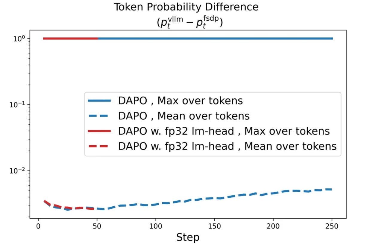
Additionally, this difference in token probabilities is not easy to fix by simply standardizing implementations across engines. Authors in [9] investigate several code interventions to decrease the gap in token probabilities with little success, and this process would have to be repeated for every combination of engines used for RL training. Instead, a more flexible approach is proposed in [9] that uses an importance sampling term to automatically correct for this engine mismatch during RL within the policy gradient expression. The exact expression is shown below and is formulated as a REINFORCE-style policy update.

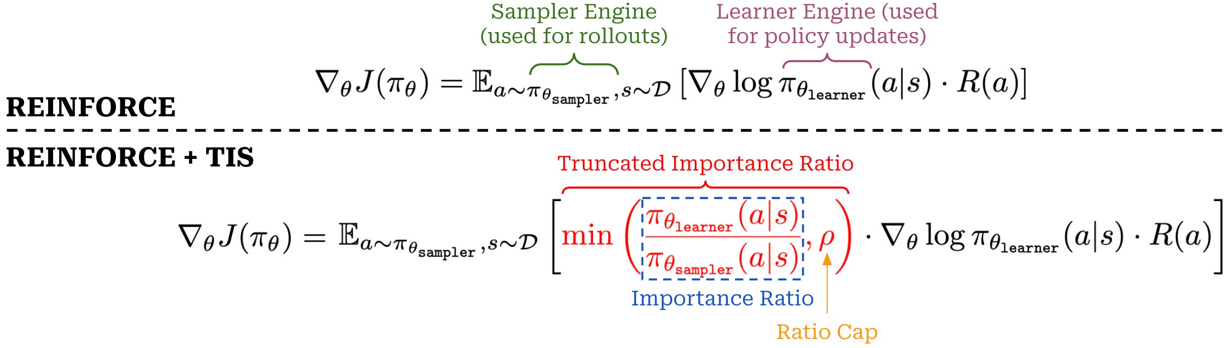
The above expression explicitly uses a different engine for sampling rollouts (sampler) and computing policy updates (learner). The importance ratio between these two engines is simply the quotient of probabilities from learner and sampler engines. In [9], authors truncate this importance ratio by capping it at a maximum size of ρ. Compared to the clipping operation used in PPO or GRPO, this truncation operation has a few differences:

• We are directly truncating the importance ratio. Clipping is also applied to the importance ratio, but it is followed by a minimum of clipped and unclipped objectives, making the operation two-sided.

• We truncate the importance ratio with a maximum value of ρ, a one-sided truncation that simply prevents extreme up-weighting.

However, the practical application of TIS is quite simple—we just compute the truncated importance ratio and multiply our policy gradient expression by this ratio. As shown below, including this importance ratio in the policy gradient has a huge impact on RL training stability and model performance, leading to quick adoption of TIS in popular training frameworks (e.g., verl and OpenInstruct).

We formulated TIS above using a sequence-level importance ratio with REINFORCE. However, we can also create a token-level formulation with PPO or GRPO; see below. As we can see, the truncated importance ratio is computed in addition to the other components of the PPO-style policy gradient expression. We then multiply the existing expression by this correction term, and this can be done either at the sequence level—similarly to the gradient expression used by GSPO—or at a token level—as in the normal expression for PPO or GRPO.

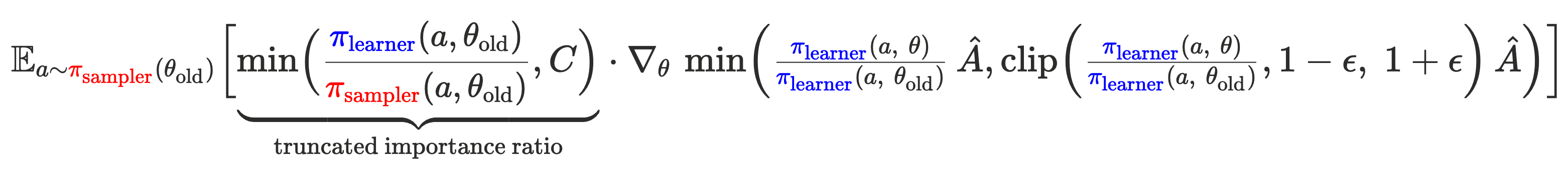
Token-level TIS is commonly used in practice due to aligning well with PPO and GRPO objectives and is, therefore, relatively simple to integrate into existing training frameworks in addition to offering stability benefits. In recent work [10], however, authors have argued from an analytical perspective that sequence-level TIS is less biased compared to token-level TIS. Currently, there is no clear consensus on which of these approaches is superior. The best implementation in practice may differ depending upon the setup or domain being considered.

Clipped Importance Sampling-Weight Policy Optimization (CISPO) [8] is another recent RL variant that, similarly to TIS, builds upon a REINFORCE-style objective with an added importance ratio. When using a PPO-style clipping approach, we know any token that is clipped from the objective has no contribution to the policy gradient. In [10], authors observe empirically that the important “fork” tokens in the model’s reasoning trace (e.g., “aha” or “wait”) are rare and are initially assigned low probabilities in the base model. Due to the importance of these tokens, their probability usually increases drastically after the first policy update, leading these tokens to have a very large importance ratio—that is then clipped by the PPO objective—for subsequent policy updates.

“We found that tokens associated with reflective behaviors… were typically rare and assigned low probabilities by our base model. During policy updates, these tokens were likely to exhibit high [importance ratio] values. As a result, these tokens were clipped out after the first on-policy update, preventing them from contributing to subsequent off-policy gradient updates… These low-probability tokens are often crucial for stabilizing entropy and facilitating scalable RL.” - from [10]

As a result, important fork tokens are usually masked from the PPO-style loss after the first policy update for a batch of data. Although this masking may not always be an issue (i.e., most standard RL setups perform only ~2-4 updates on each batch of sampled data), MiniMax-M1 performs 16 policy updates for each batch of data. Therefore, important tokens being masked out of the loss after only one or a few updates can significantly damage training efficiency. To solve this issue, authors adopt the modified REINFORCE-style loss shown below. As we can see, CISPO adopts some of the recommendations proposed by DAPO [6] as well, including the token-level loss formulation to correct for length biases.

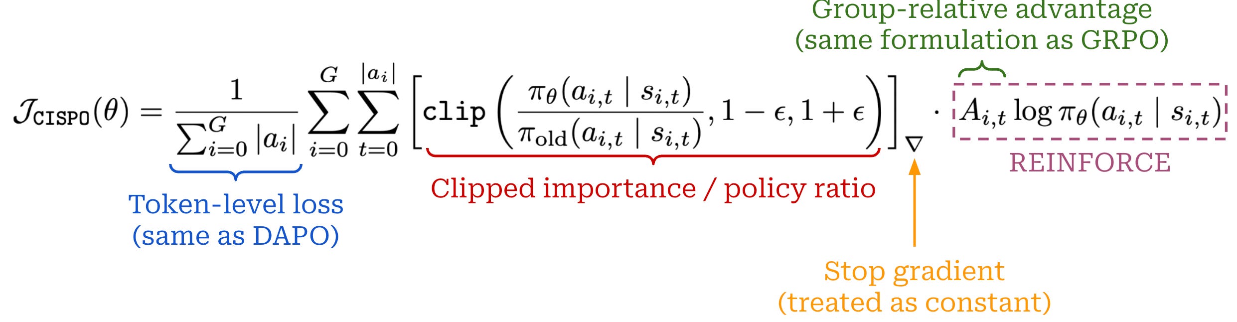
This loss formulation applies a stop gradient to the clipped importance ratio, ensuring that each token contributes to the loss even when it is clipped. Put differently, the importance ratio is used as a weight that controls the contribution of a token to the policy gradient. Clipping in CISPO puts a cap on this weight, ensuring no single token is over-amplified due to a large importance ratio.

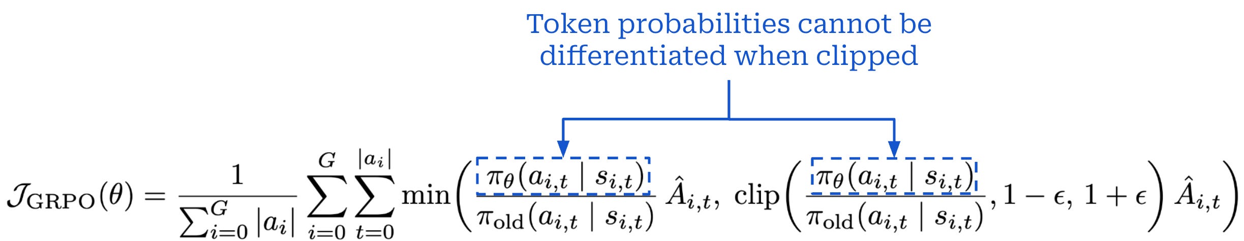
When we look at the GRPO objective, the clipping mechanics are quite different; see above. In particular, token probabilities are only present in the importance ratio, and the gradient flows through the token probability terms inside the importance ratio. When the importance ratio is clipped, the gradient for that token is zero and there is no contribution to the policy gradient. The modified clipping approach used by CISPO ensures that all tokens contribute to the policy gradient, improving the stability and efficiency of RL; see below.

The loss formulation of CISPO and TIS look quite similar, but these algorithms—despite both using an importance ratio—aim to solve different issues. CISPO uses the same definition of the importance ratio adopted in PPO and GRPO. This importance ratio is clipped to ensure that token probabilities do not change too much over a single batch of data, thus enforcing a trust region. CISPO simply modifies the manner in which the importance ratio is clipped to ensure that all tokens continue contributing to the policy gradient (with a capped weight) even if they are clipped. On the other hand, TIS uses an importance ratio to capture the difference in token probabilities between training and inference engines, thus correcting for the mismatch between engines during RL training.

Further reading. For more details on each of these algorithms, please see the overview linked below, which covers many GRPO variants and modifications.

There are two primary regularization terms commonly added to RL training:

1. Entropy bonus: rewards the LLM for remaining uncertain and helps to avoid overly-confident token distributions.

2. KL divergence: anchors the policy to a reference policy throughout training to prevent the LLM from changing too much.

Regularization terms are less commonly used in recent RL training pipelines, but we will see examples of both strategies being applied later in the overview. To avoid future confusion, we will briefly explain each regularization strategy now.

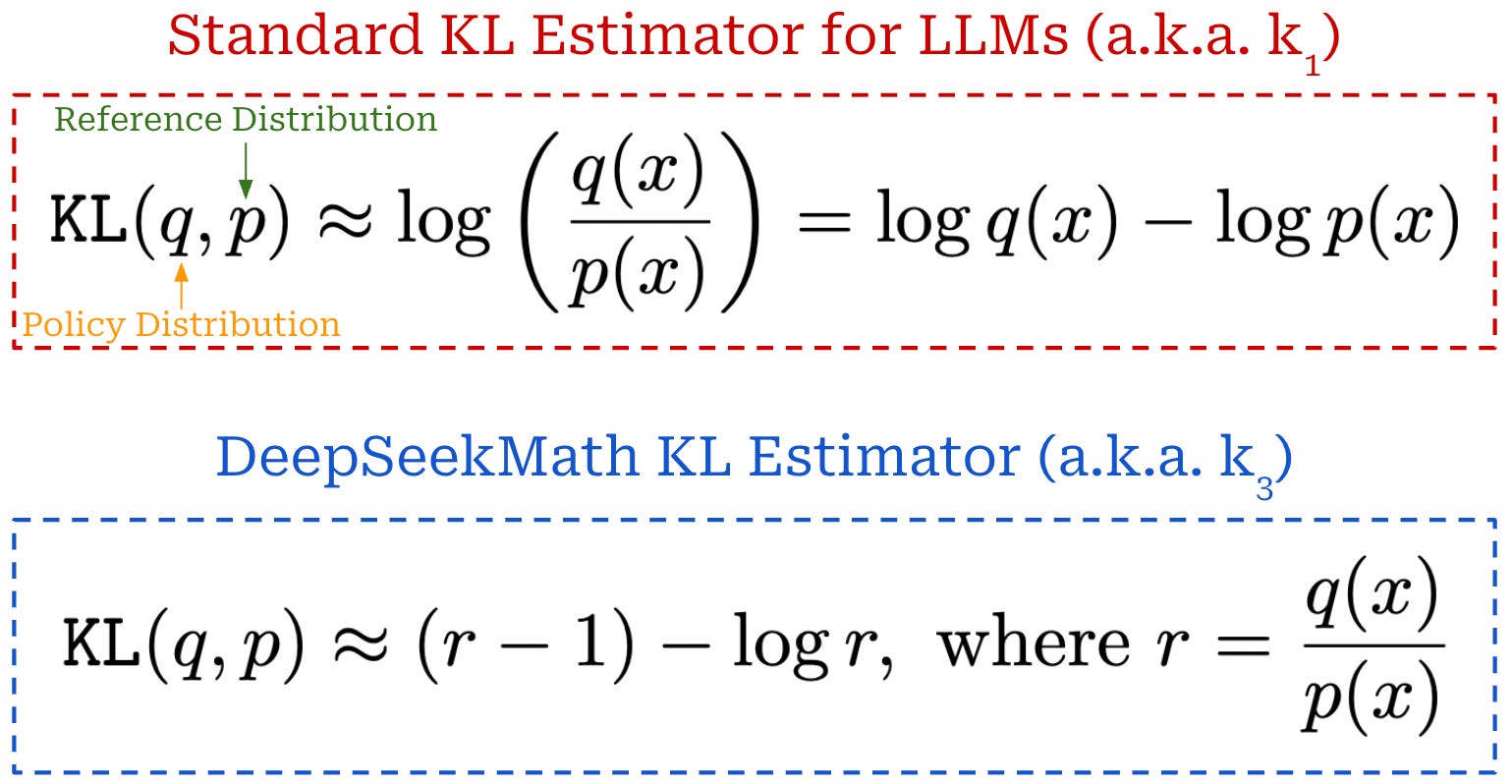
KL divergence. During RL training, we can compute the Kullback-Leibler (KL) Divergence between the current policy and a reference policy—usually the policy from before RL training begins (i.e., the base model). There are several techniques that can be used to approximate the KL divergence between two models; see here. The easiest—and most common—approximation of KL divergence [7] is the difference in token-level log probabilities between the current policy and the reference policy. This approximation and another common variant used in the original GRPO paper [12]4 are outlined below. Both estimators are usually supported in open RL implementations; e.g., see their implementation in TRL.

After the KL divergence has been computed, there are two common ways that it can be incorporated into the RL training process:

1. By directly subtracting the KL divergence from the reward.

2. By adding the KL divergence to the loss function as a penalty term.

Both of these approaches can be found in practice depending on the RL optimizer—or exact implementation—being used. PPO incorporates KL divergence into the reward, while GRPO adds it as a penalty to the objective function; see below.

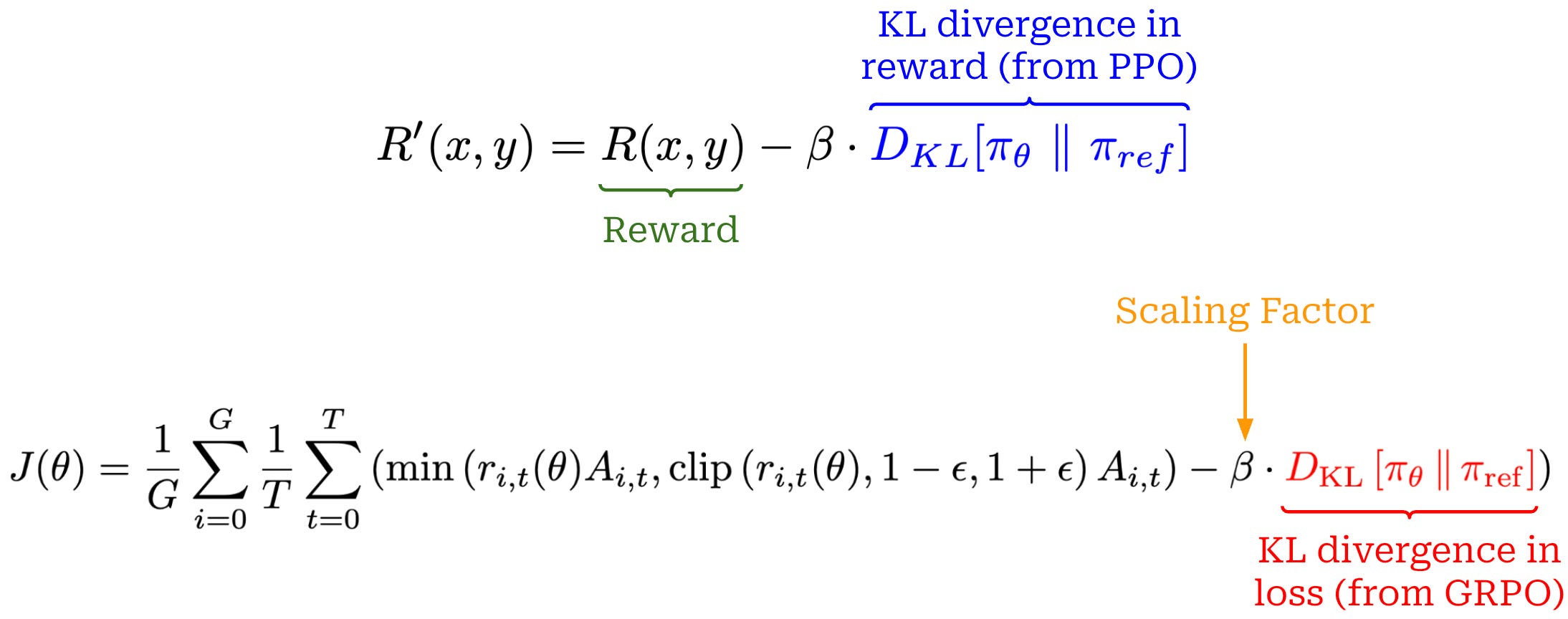
Due to the popularity of GRPO, recent RL implementations more often include the KL divergence in the loss, but completely omitting the KL divergence—and not using any regularization—is becoming increasingly common. During training, the KL divergence term penalizes our policy from becoming too different from the reference policy, but drifting away from the reference policy may not be negative if we are performing large-scale, reasoning-oriented RL training.

Entropy bonus. From an information theory perspective, entropy captures the level of uncertainty associated with the possible states for a variable:

• High entropy: probability mass is spread across many outcomes.

• Low entropy: probability mass is concentrated on a few outcomes.

In the LLM domain, we can measure the entropy of a model’s token distribution—low entropy means that the LLM places most of its probability into a small set of tokens and vice versa. Specifically, we can compute entropy using the equation below.

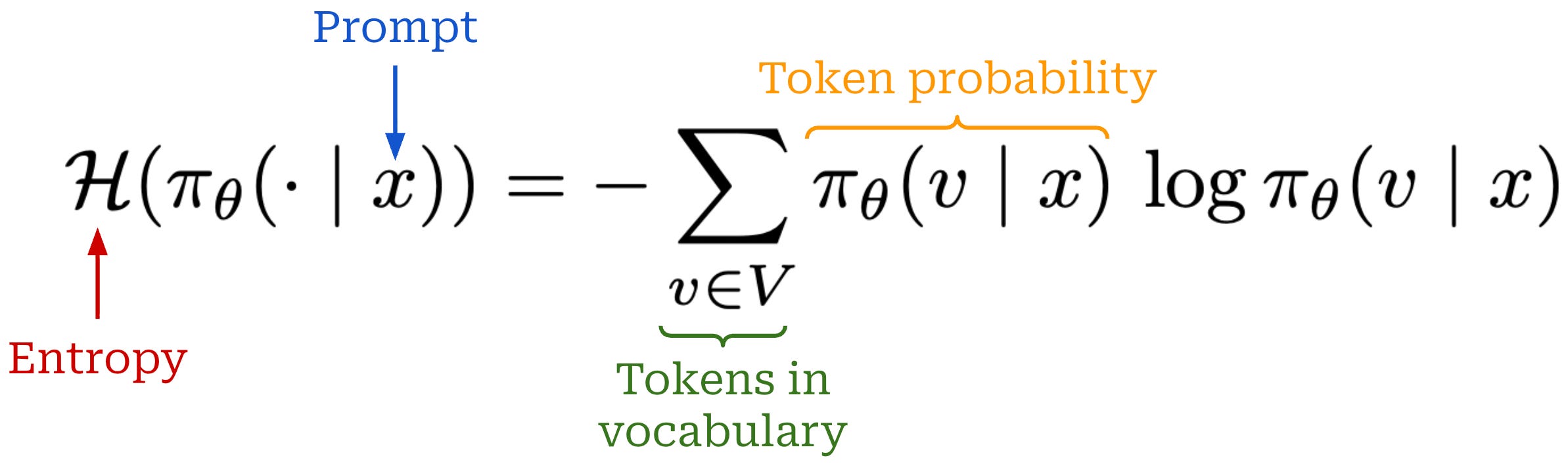
Usually, entropy is computed for each token (i.e., at each decoding step) and then averaged across the generated trajectory. After computing the entropy, we can turn it into an entropy bonus and use it as a regularization term by simply scaling it with a coefficient β and incorporating it into either the reward—this is done in the original PPO paper—or the objective function. The purpose of the entropy bonus is to prevent the LLM from becoming overly confident in its token distribution and, in turn, avoid entropy collapse that prevents the policy from exploring during training. Similarly to the KL divergence, entropy bonuses are now more commonly incorporated into the loss function. In fact, we will soon study a paper that adds an entropy bonus to the GRPO loss [3].

“While RL compute for LLMs has scaled massively, our understanding of how to scale RL has not kept pace; the methodology remains more art than science.” - from [1]

Scaling laws provide researchers with the ability to extrapolate the performance of expensive training runs from those that require less compute. Despite the expanding role of RL in training frontier models, however, our understanding its fundamental scaling properties remain somewhat rudimentary, especially relative to pretraining. In this section, we will take a look at several notable papers that are trying to solve this issue. As we will see, RL scaling laws are very different from those used for pretraining, and many of these differences arise from the massive design space of RL training. Put simply, RL is complicated, and we are far from a single standardized approach for handling RL “correctly”. However, there are still useful scaling insights that can be gleaned from this work that will help us to allocate available compute for RL experiments more effectively.

Unlike pretraining, RL has no established predictive scaling laws for reliably estimating performance trends. Best practices for RL are found in new algorithm proposals, but these findings may not generalize at scale. Model reports also frequently provide practical recommendations for RL training, but these methods are often anecdotal and dependent upon training settings. As a result, we must test RL design choices the hard way—by running large-scale experiments and seeing what works. Given the computation cost of modern RL, this approach is a major bottleneck that limits iteration speed and hinders technical progress. We need a standardized approach to identify strong RL candidates at smaller scales.

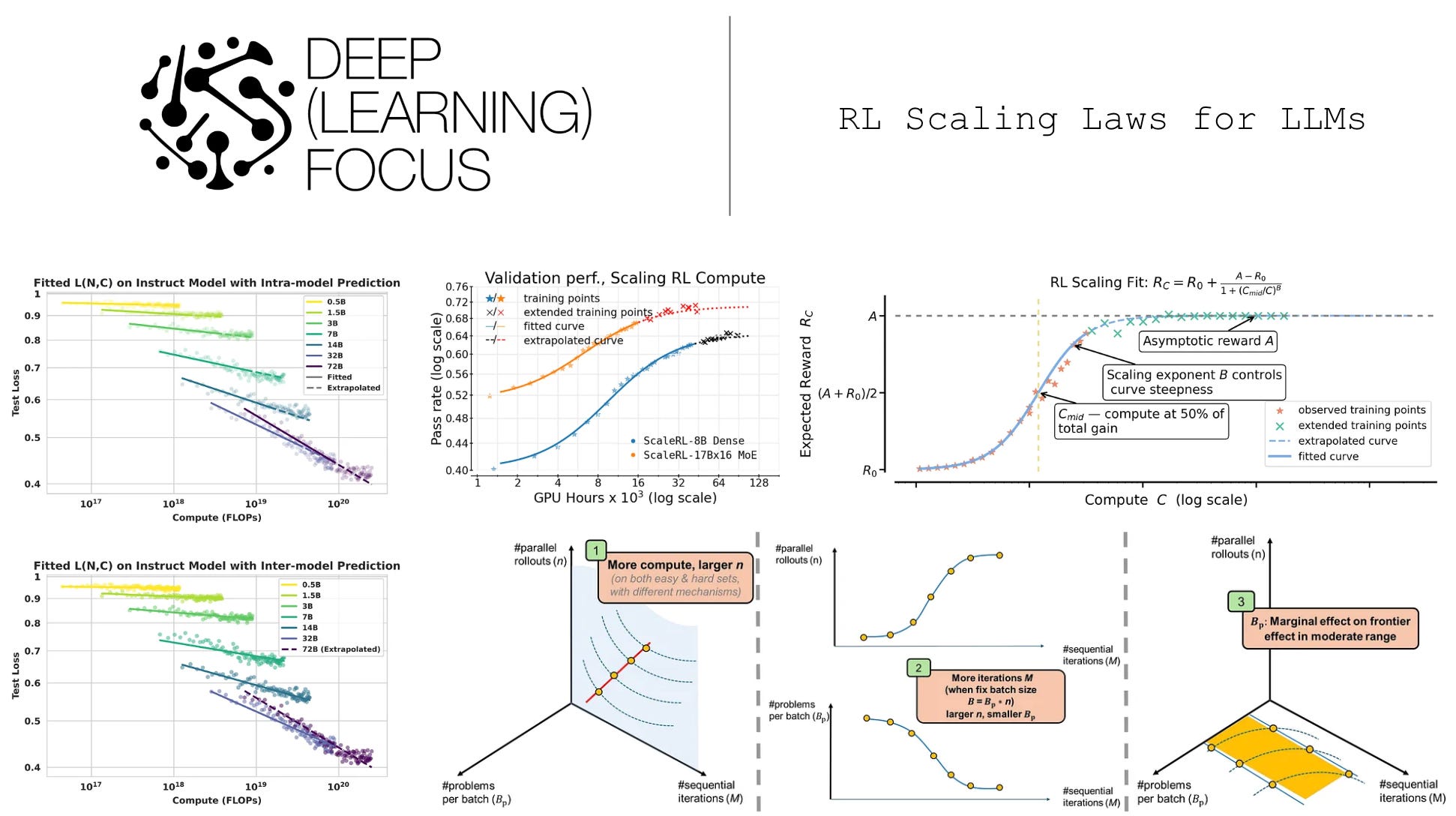
RL scaling. In [1], authors model the RL training process with sigmoidal compute-performance curves. We fit such a curve separately for each RL training run to model the relationship between expected reward—calculated over a validation set at regular intervals during training—and compute (in units of GPU hours); see below.

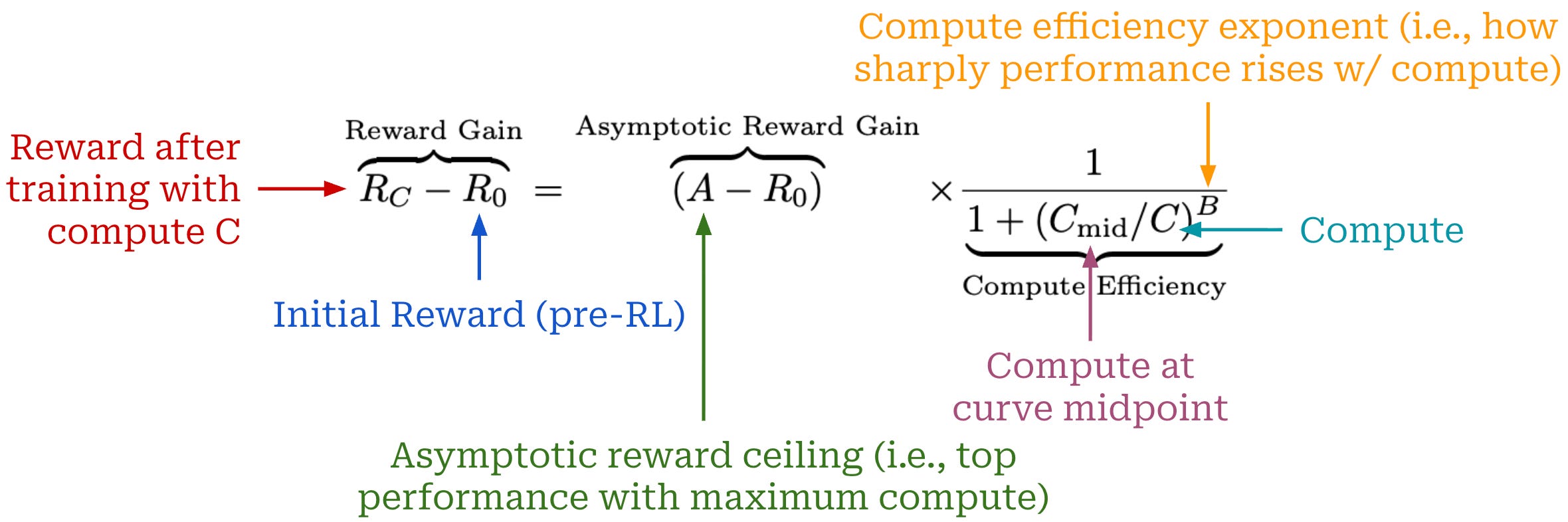
This curve models the relationship between two quantities:

1. Reward gain: the difference between the reward after RL training with compute C and the initial reward before RL training.

2. Asymptotic reward ceiling: the maximum possible gain in reward we can achieve by spending unlimited compute on RL training.

The relationship between these quantities is controlled by the term 1 / [1 + (C_mid​/C)^B​]. This term includes i) the compute level at which we reach the midpoint of the curve C_mid, ii) an efficiency exponent B for the steepness of the curve, and iii) the current compute level C. Intuitively, this term captures how much of the total possible performance gain has been unlocked by running RL with compute C. The shape of this curve is visualized in the figure below.

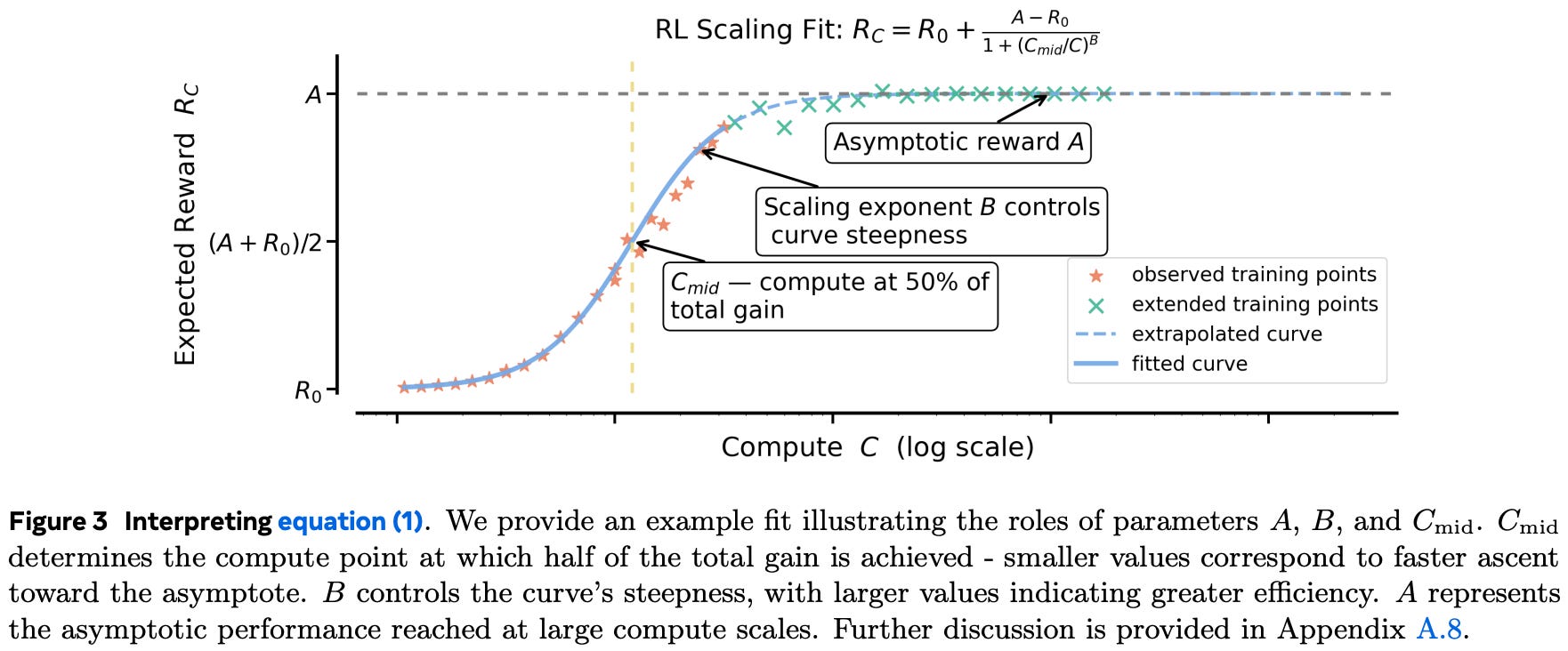
According to this structure, RL training is flat in terms of reward during the early phase of training, then undergoes a phase of fast improvement before reaching a plateau. Authors find in [1] that these saturating curves between compute and reward robustly model the RL training process in practice. As we will see, this structure has also been validated and adopted by other work on RL scaling.

We fit this curve to the results of each RL training run, allowing us to compare results obtained from multiple runs with different training setups. There are two ways that these scaling curves may differ:

1. Their value of A may be different, indicating that one training setting achieves better asymptotic performance.

2. Their value of B (or C_mid) may be different, meaning that one training setting is more compute efficient than the other.

However, not all training settings yield a benefit in both A and B. In such cases, authors prioritize asymptotic improvements over efficiency improvements, arguing that improving the model’s asymptotic performance is more valuable because a degradation in efficiency can be offset by just training for longer.

Applying RL scaling laws. The RL scaling laws proposed in [1] allow us to extrapolate the performance of a training run without incurring the full cost. We can use the early phase of training to predict what would be the final performance after training with more compute. The scaling law is fit using validation performance measured at regular intervals during training5, allowing us to efficiently assess the scalability of different changes to the RL training process.

“We propose a best-practice recipe, ScaleRL, and demonstrate its effectiveness by successfully scaling and predicting validation performance on a single RL run scaled up to 100,000 GPU-hours. Our work provides both a scientific framework for analyzing scaling in RL and a practical recipe that brings RL training closer to the predictability long achieved in pre-training.” - from [1]

Authors in [1] use this approach to derive an optimal training recipe, called ScaleRL. Beginning with a baseline setup, authors test interventions to the RL training process in multiple phases of increasing scale—4K, 8K, 16K, and 100K GPU hours. In each phase, scaling laws are fit to extrapolate the performance of each setting, allowing authors to both i) verify the accuracy of their scaling law formulation and ii) efficiently discover scalable design choices for RL.

“We present the first large-scale systematic study, amounting to more than 400,000 GPU-hours, that defines a principled framework for analyzing and predicting RL scaling in LLMs.” - from [1]

Baseline RL setup. RL experiments in [1] primarily use the Polaris-53K math-focused reasoning dataset. Analysis begins with a baseline RL recipe that uses the GRPO loss with no KL divergence and the clip higher approach from DAPO [6]. All models produce a reasoning trace before their final output. A context length of 16K tokens is used—12K reasoning tokens, 2K input tokens, and 2K output tokens—as well as a batch size of 768—a total of 48 prompts with 16 rollouts each.

To enforce the 12K-token reasoning budget, interruptions are used during training. When a reasoning trace reaches 12K tokens, we append a static end-of-reasoning phrase “Okay, time is up. Let me stop thinking and formulate a final answer. </think>" to the model’s output so that the model can stop reasoning and begin generating a final answer.

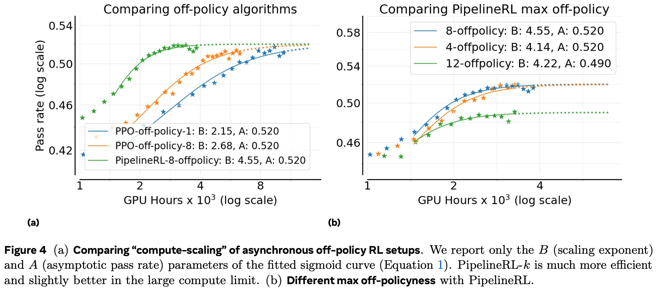
From an engineering perspective, authors adopt a split generator-trainer approach, where a subset of GPUs run optimized inference engines (e.g., vLLM) for generating rollouts and remaining GPUs run a training backend (e.g., FSDP) to update policy parameters. To improve efficiency, an asynchronous RL training approach is adopted. Two algorithms are considered: asynchronous PPO and PipelineRL [11]. As shown above, both approaches achieve similar asymptotic performance A, but PipelineRL has significantly improved compute efficiency B due to its design principles that minimize GPU idle time (e.g., in-flight weight updates). Authors also find in [1] that it is important to bound the degree of asynchrony by ensuring policy updates are not more than K steps ahead of the generated rollouts. K = 8 is found to be optimal for this setting; see above.

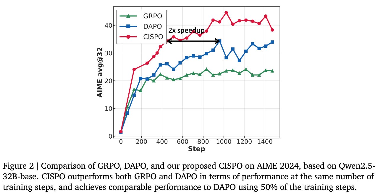
Ablating RL modifications. To build upon the baseline RL recipe, authors run small-scale RL experiments (i.e., ~4-8K GPU hours) to test the impact of various RL design choices. The baseline loss is first compared with both GSPO and CISPO loss formulations; see below. We see that both GSPO and CISPO noticeably outperform the baseline formulation in terms of asymptotic performance. CISPO also has marginally improved compute efficiency relative to GSPO, leading authors to use CISPO for remaining experiments in [1].

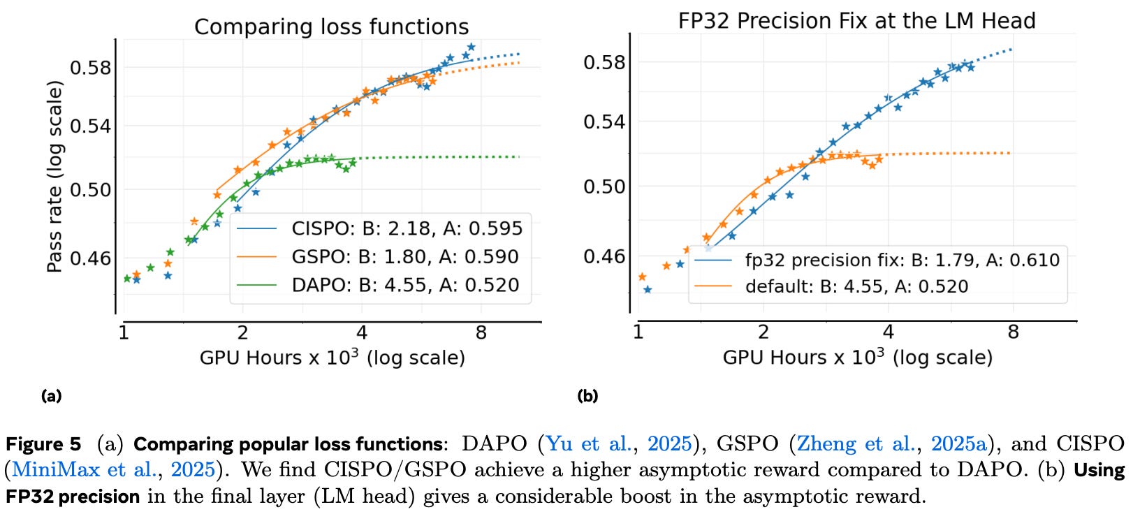
As we learned from the explanation of TIS, using different engines for generating rollouts and computing policy updates can lead to a non-negligible mismatch in log probabilities between training and inference. One change that we can make to minimize this mismatch is using full (float32) precision in the LLM’s language modeling head—the final linear layer that predicts token probabilities. As shown above, using a full precision head in training and inference engines significantly improves both asymptotic performance and compute efficiency. We should note, however, that authors do not adopt any approach for correcting the trainer-generator mismatch (e.g., TIS), which could also help to solve this issue.

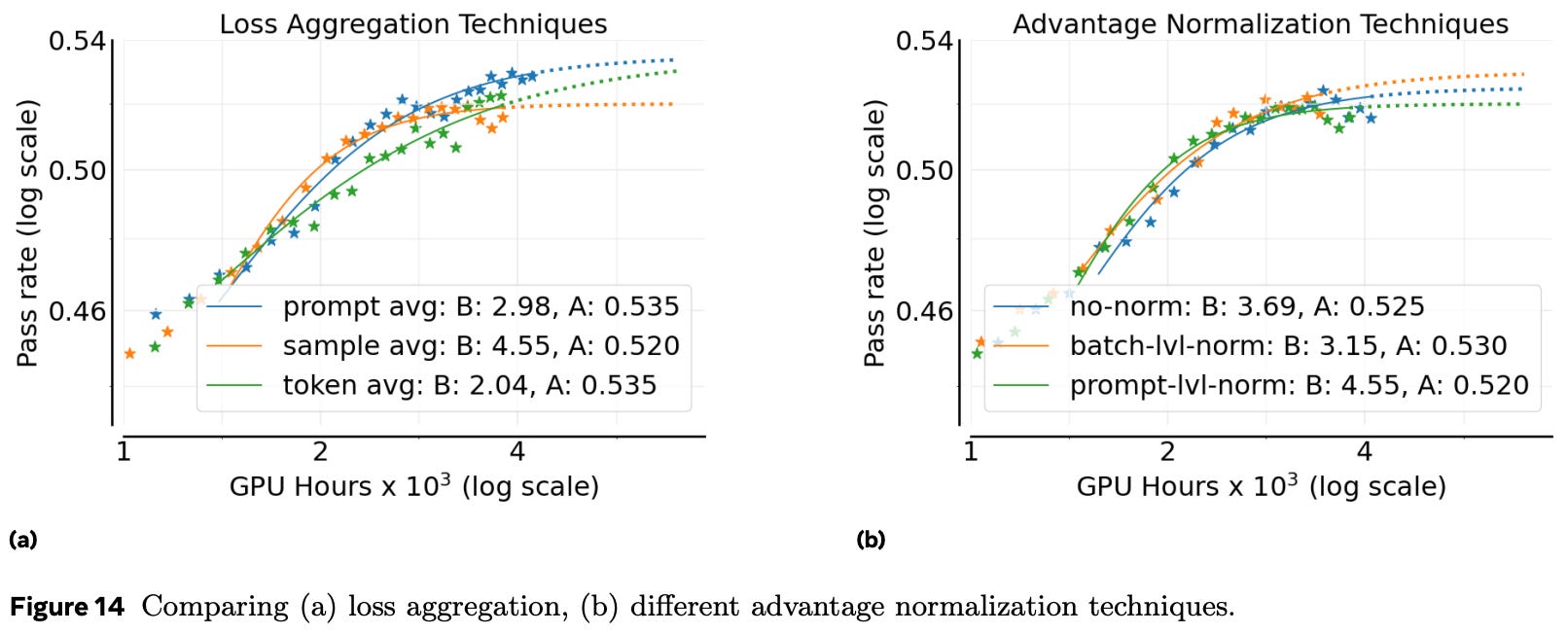
Authors also test different loss aggregation strategies, including vanilla GRPO aggregation versus DAPO-style aggregation, finding that the loss aggregation proposed by DAPO [6] tends to perform the best; see below. In a similar vein, several advantage normalization techniques are tested. Specifically, authors test dividing mean-centered rewards by the standard deviation of rewards in a group—as in vanilla GRPO—or the standard deviation of rewards in the entire batch, as well as not dividing the mean-centered reward by anything—as in Dr. GRPO [7]. All techniques perform comparably, indicating that advantage normalization does not significantly impact asymptotic performance; see below. Remaining experiments normalize the advantage using the standard deviation of rewards across the batch due to the slight boost observed in asymptotic performance.

Authors also discover data curation and filtering strategies that benefit the asymptotic performance of RL. Prompts with zero variance in rewards across a group have zero advantage and, therefore, no contribution to the policy gradient. Filtering these zero variance prompts from the batch benefits asymptotic performance; see below. Notably, this approach is different from the dynamic sampling method proposed in DAPO [6], as we do not continue sampling prompts until the batch is full. Rather, we just filter zero-variance prompts from the batch, forming a smaller effective batch. By doing this, we avoid dampening the policy gradient signal, as we are averaging the policy gradient over a smaller effective batch instead of the full batch that includes prompts with no gradient.

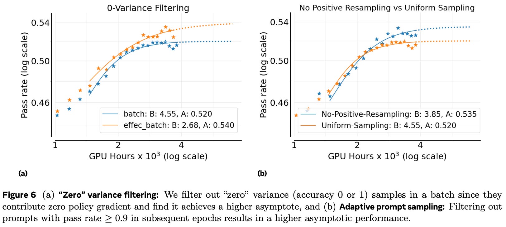
Many data curriculum strategies have been proposed for RL training, but we learn in [1] that simple approaches can be quite effective. During training, the number of prompts that are solved easily by the current policy increases, and these prompts usually remain easy for the model throughout the rest of training. As shown above, dynamically removing these prompts from the training process improves asymptotic performance. To do this, authors maintain a history of pass rates for each prompt and permanently remove prompts that exceed a pass rate of 90%. This approach, called no positive resampling in [1], avoids wasting compute on prompts that the model already knows how to correctly solve.

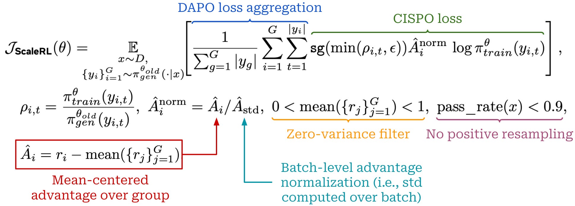
The ScaleRL recipe, which combines all best practices identified in the smaller-scale experiments outlined above, uses the loss formulation shown above. As mentioned before, a PipelineRL setup, forced interruptions for reasoning, and a full precision language modeling head are also used for ScaleRL.

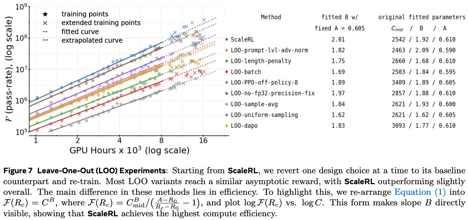
To validate this recipe, larger-scale experiments are performed with up to 16K GPU hours. Authors perform leave-one-out ablations by removing individual components of the ScaleRL recipe to determine if they still have an impact when used in tandem with other components. When fitting sigmoidal scaling curves up to 8K GPU hours, we see that extrapolated results accurately predict performance up to the end of the 16K GPU hour run. In these experiments, the full ScaleRL recipe is found to yield the best performance; see above. Not all components significantly benefit performance in the leave-one-out analysis, but authors argue that these design choices still tend to benefit training stability.

“Even when individual design choices appear redundant within the combined recipe, they often enhance training stability, robustness, or efficiency in ways that generalize across models and setups. ScaleRL retains such components not just for marginal gains in a specific configuration, but because they address recurring sources of instability and variance that arise across RL regimes.” - from [1]

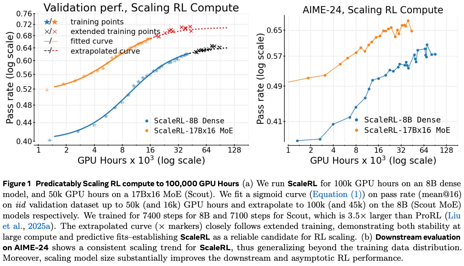
Scaling up. Based on the analysis in [1], authors perform a final training run of ScaleRL up to 100K GPU hours, finding that the extrapolated performance continues to match actual performance in extended RL training runs; see below. Prior to this large-scale experiment, different methods for scaling up the RL training process (e.g., longer context, larger batch size, larger models, etc.) are considered in [1]. By analyzing these options in this extended run of ScaleRL, we learn the following:

• The scaling laws proposed in [1] are also found to accurately extrapolate the performance of Mixture-of-Experts models, indicating generalizability to larger models with different architectures.

• Using a longer context window during RL slows down training progress initially but yields higher asymptotic performance in the long run.

• Increasing the batch size improves the asymptotic performance of RL and prevents stagnation on downstream benchmarks.

• How we allocate the batch in terms of number of prompts and number of rollouts per prompt is less impactful—the total batch size matters most.

Key takeaways. The empirical analysis in [1] is extensive and contains a wide variety of practical details that are incredibly useful for those working on RL. For this reason, those who are interested in gaining a practical grasp of RL training should definitely read the full paper. However, the comprehensive empirical analysis presented in [1] can be largely summarized as follows:

• Asynchronous RL (i.e., PipelineRL) with a split generator-trainer setup is highly efficient and yields models that perform well, so long as we bound the level of asynchronicity during training.

• The proposed ScaleRL training recipe combines all of the practical GRPO modifications that were found to be useful across experiments in [1].

• The performance ceiling of RL A can be impacted by changes to the RL setup (e.g., loss type or batch size). However, many common RL interventions (e.g., loss aggregation, data curriculum, or advantage normalization) impact compute efficiency B rather than asymptotic performance.

• The methods that appear superior in smaller-scale RL runs do not always generalize to the high-compute regime. However, we can still identify the recipes that are most scalable by fitting a sigmoidal scaling curve and estimating scaling parameters A and B from early training dynamics. This approach is used constantly throughout the analysis in [1] to judge the scalability of RL recipes without performing full training runs (i.e., 16K-100K GPU hours).

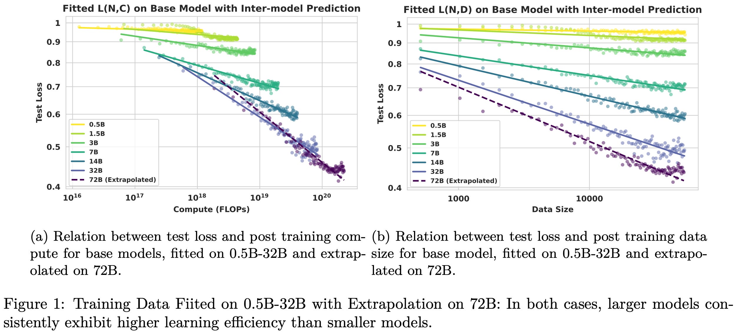
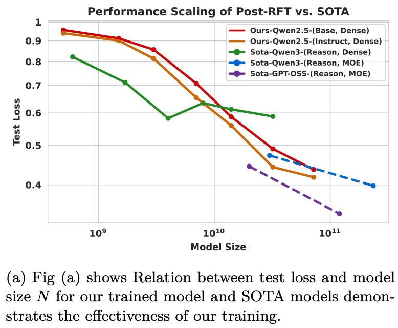
In [2], authors investigate scaling behaviors of RL post-training using the full Qwen-2.5 model suite—both base and instruct models—ranging from 0.5B to 72B parameters. As in [1], this paper studies the impact of factors like model size, data volume, and compute on the performance of models trained with RL. However, this analysis focuses specifically on the mathematical reasoning domain, uses only the vanilla GRPO algorithm, and adopts a different scaling formulation. From the analysis in [2], we learn that RL follows a predictive power-law relationship between test loss and compute or data; see above.

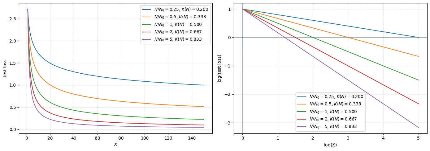
Scaling formulation. The scaling law formulation in [2] fits a relationship between test loss—defined as the error rate (i.e., error rate = 1 - accuracy) on an in-domain validation set—and compute or data. As shown below, RL scaling behavior is modeled using a log-linear power law between the test loss L, model size N, and a resource budget X. Here, the resource budget can either be the amount of compute C or the amount of data D used during RL training.

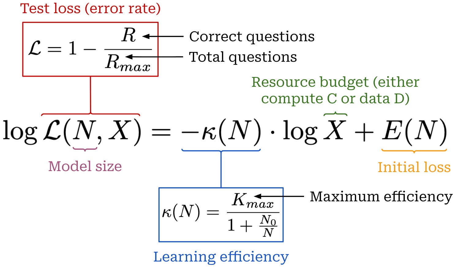
In the figure below, we plot this power law—using both log-log scale and linear scale to make interpreting the plots easier—for different values of the learning efficiency. We use a fixed value of E(N) = 1.0 in this plot for simplicity. As we can see, performance improves log-linearly as the resource budget X increases, and higher learning efficiency K(N) leads to a steeper decrease in test loss.

Performance extrapolation. As we might have inferred, the scaling formulation used in [1] is quite different from the pretraining scaling laws that we learned about before. More specifically, the scaling trends in [1] can only extrapolate the results of a specific training run to a higher compute regime—we are predicting what will happen if we continue the RL training process for longer. In contrast, the power law in [2] enables multiple extrapolation regimes:

1. Inter-model: fit the scaling law using data from training runs with smaller models (i.e., 0.5B to 32B Qwen-2.5 models) and predict the performance of a larger model (i.e., Qwen-2.5-72B).

2. Intra-model: fit the scaling law using the early training trajectory of a model and predict its performance for the remainder of training.

Both kinds of extrapolation are validated in [2] across base and instruct model variants of several sizes, demonstrating that RL training follows predictable scaling trends across model size N, compute C, and data volume D. Scaling plots shown in [2] always provide both inter and intra-model extrapolation results.

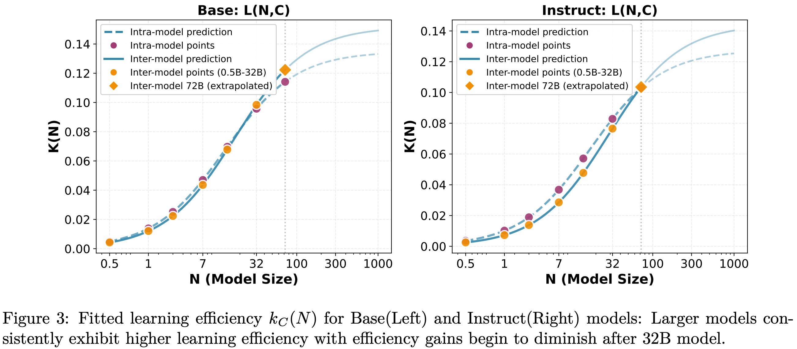
More on learning efficiency. In our above scaling law expression, we should notice that the learning efficiency term has a dependence upon N—learning efficiency follows a saturating trend with model size. Put simply, this means that i) larger models have higher learning efficiency, but ii) marginal efficiency gains begin to diminish with increasing model size. As shown in the plot below, this formulation matches empirical observations. In practice, learning efficiency follows a saturating S-curve—similar in structure to the scaling law formulation proposed in [1]6—that plateaus at a maximum learning efficiency of K_max.

Experimental setup. All experiments in [2] use vanilla GRPO—with a KL divergence term—and the verl training framework. Scaling laws are empirically fit and validated on results from over 60 models, including base and instruct variants from the Qwen-2.5 series with sizes ranging from 0.5B to 72B parameters. The model family is fixed to ensure that only parameter count N and data volume D are changing. RL training is conducted over 50K samples taken from the mathematics subset of guru-RL-92K, which performs extensive deduplication and difficulty filtering. Additionally, authors in [2] sort problems by increasing difficulty—as assessed by the pass rate of Qwen2.5-7B-Instruct—to form a data curriculum of increasing problem difficulty as RL training progresses. Following standard practice for fitting scaling laws, we compute test loss on an in-domain dataset of 500 held-out problems sampled from the training distribution.

Compute-constrained regime. The power law formulation in [2] can be used to characterize scaling behavior under a fixed compute budget. Given a compute budget C, we are interested in the optimal model size N that minimizes the test loss. In [2], the compute budget is estimated via cumulative training FLOPs C = 6 × N × T, where T is the number of tokens processed during training. T is related to the data volume D, but whereas D counts data samples, T measures the total token volume. T is inferred from fixed values of C and N. We can study the relationship between compute C and model size N by running RL training with various model sizes and compute budgets, then fitting scaling laws on the results. We use compute as our resource budget (i.e., X = C) for these scaling laws; see below.

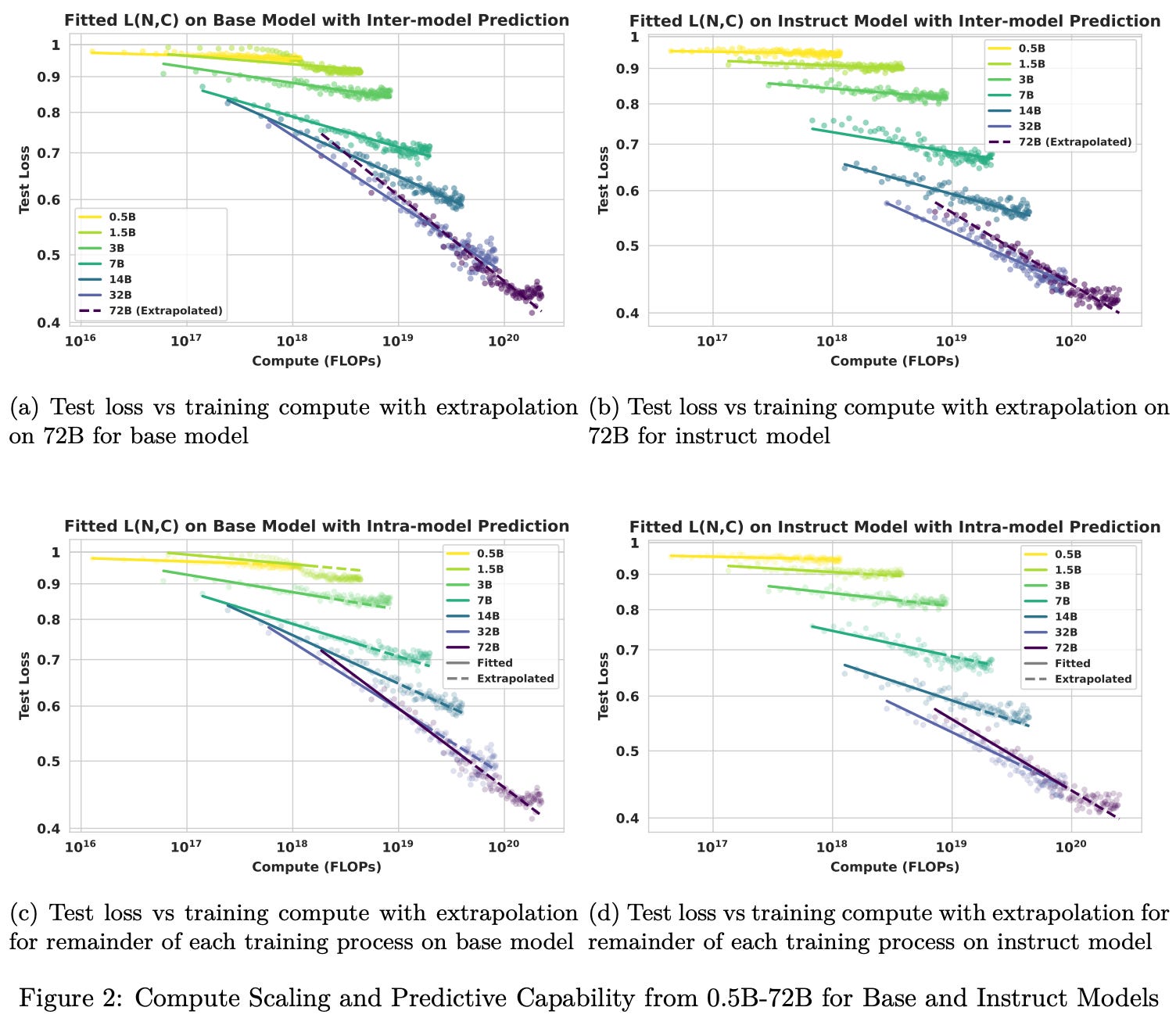
In these plots, we can observe the results of inter-model (top plot) and intra-model (bottom plot) extrapolation using the scaling law formulation proposed in [2]. When studying scaling trends for smaller models (i.e., 0.5B to 32B parameters), we see that the best performance under a fixed compute budget is usually achieved by using the largest model. Larger models (i.e., 32B and 72B parameters) violate this trend: the 32B model performs best at lower compute budgets, but a crossover occurs at higher compute budgets after which the 72B model performs better.

“In contrast to the immediate dominance of larger models in smaller parameter regimes, the 32B model outperforms the 72B counterpart initially under equivalent compute budgets, as the smaller model size inherently enables more training steps. We believe this observation reveals a latent trade-off between model scale and training steps in compute constrained scenarios.” - from [2]

This crossover arises from the fact that learning efficiency k(N) saturates for larger models. Given a fixed compute budget C, a smaller model can train for a larger number of steps relative to a larger model. Therefore, the larger model must have significantly improved learning efficiency in order to outperform the smaller model. As we see in the scaling analysis above, this is true until we reach 72B scale, at which point efficiency gains saturate and the 32B model is able to exceed the performance of the larger model under tight compute constraints.

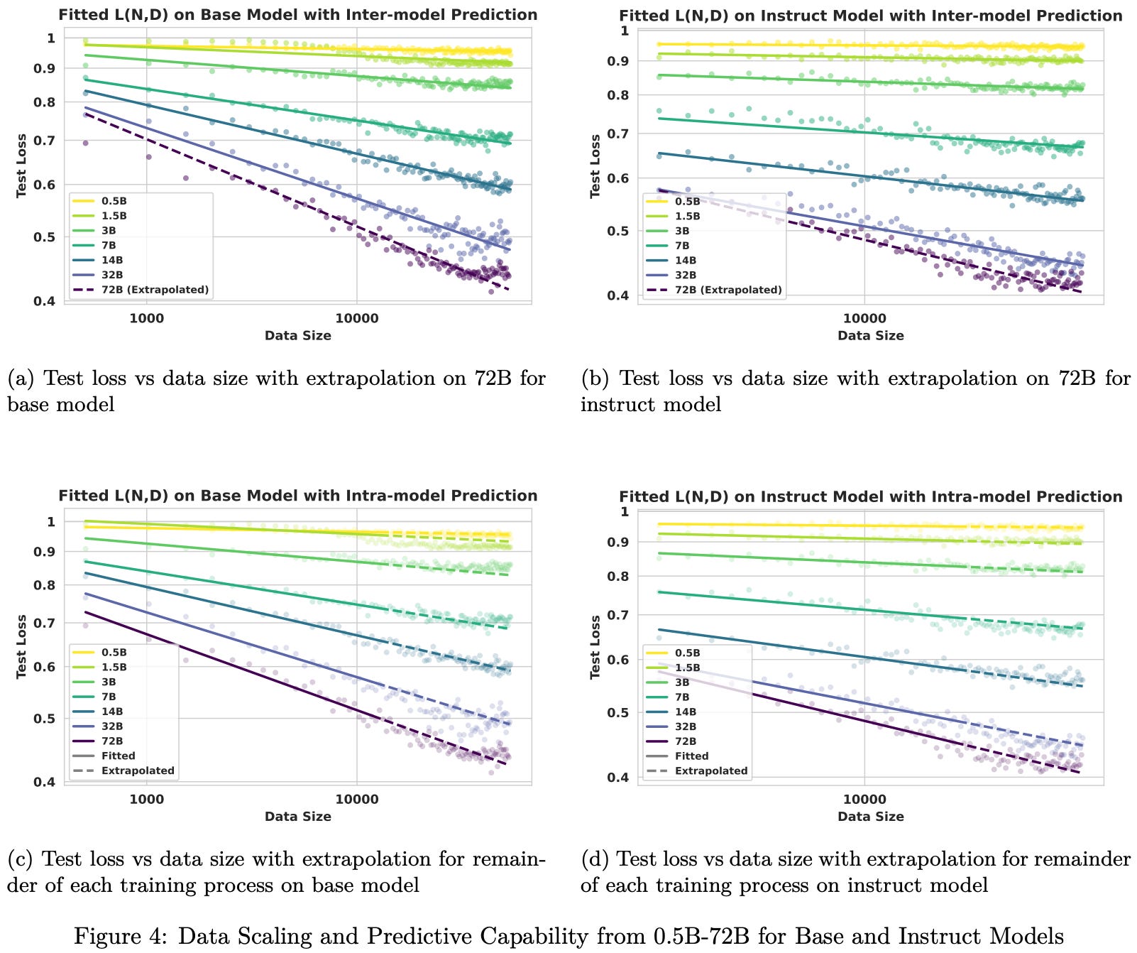
Data-optimal scaling. Given that LLM training is usually bottlenecked by the availability of high-quality data, we also want to understand the optimal model size for RL training given a fixed data budget D7. To do this, we can train models with various model sizes N and data budgets D, then fit the scaling laws—where data is our resource budget (i.e., X = D)—to these results; see below. The conclusion from this analysis is simple: for a fixed amount of data, larger models demonstrate superior sample efficiency and consistently achieve lower test loss. We also see that scaling laws accurately extrapolate performance in all regimes considered.

If we remove data and compute constraints (i.e., train models to convergence on sufficiently large datasets), test loss monotonically decreases with model size—bigger models are better given enough data and compute. However, this trend does not follow a power law; see below. Smaller models show weaker gains, indicating diminishing returns for training smaller models to convergence.

Data reuse. In addition to the scaling analysis, authors in [2] test if repeating data during training is problematic. These experiments fix the total data budget D_total but vary the number of unique data samples such that D_total = τ × D_unique, where τ is a data reuse factor. As shown below, we learn in [2] that performance is primarily determined by D_total rather than D_unique. In fact, test loss is relatively insensitive to τ, and we see that there is no significant degradation in performance until larger reuse factors (i.e., τ = 25).

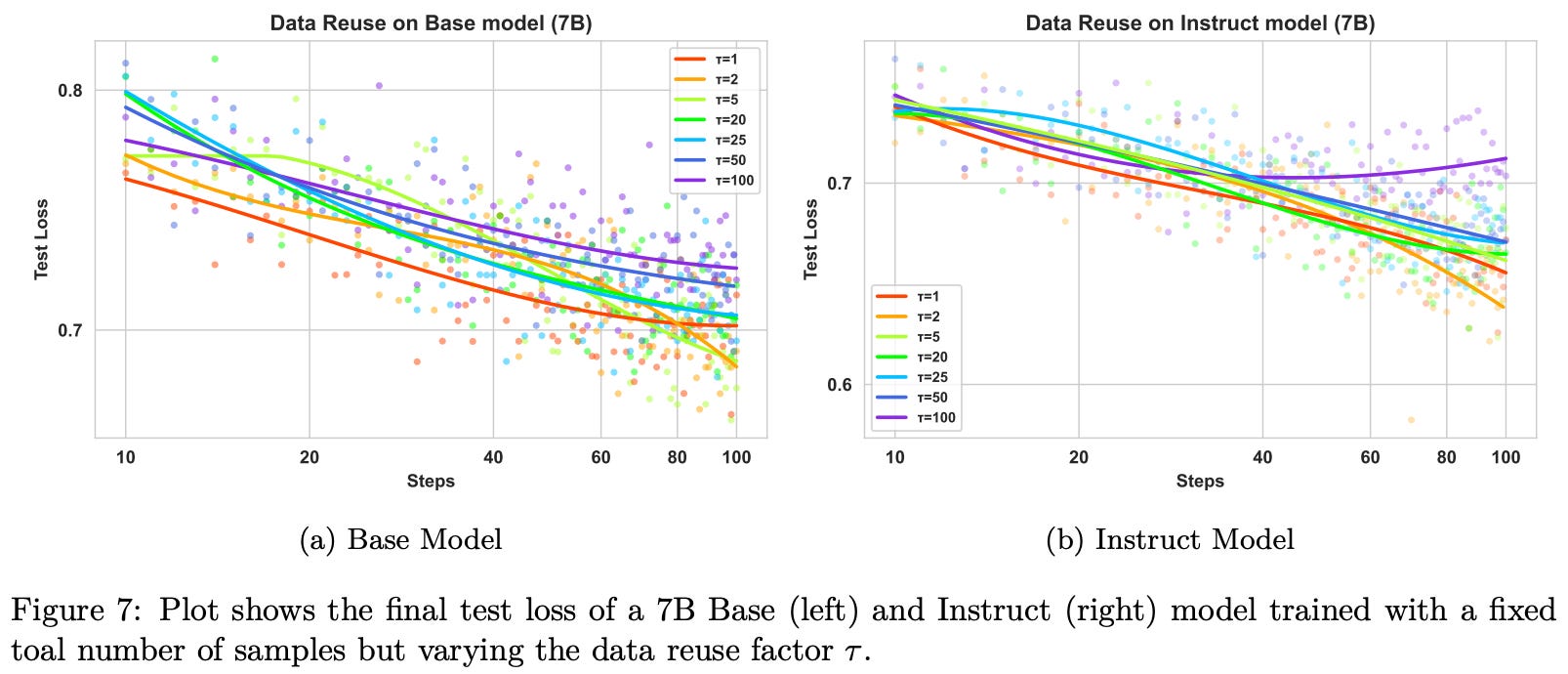
However, unique data is not sampled randomly in these experiments. To ensure that data subsets are sufficiently diverse, authors partition the training set into difficulty subsets and preserve the data difficulty distribution across subsets of different sizes. Additionally, the same data curriculum is maintained by ordering data based upon difficulty. The robustness of RL training to data reuse is likely dependent upon the diversity, quality, and difficulty of the unique samples.

Scaling laws can be applied to RL training in many ways. The work we have seen so far shows that performance during RL follows a sigmoidal trajectory [1] and scales in a predictable manner with model size under fixed compute budgets [2]. However, these results, while informative, do not directly recommend how we can practically allocate a fixed compute budget for RL training in a similar manner to pretraining scaling laws. Inspired by this, authors in [3] perform a prescriptive analysis of optimal compute allocations for RL. Specifically, the analysis in [3] focuses on understanding how to optimally allocate sampling compute—or the amount of compute spent generating completions for on-policy RL.

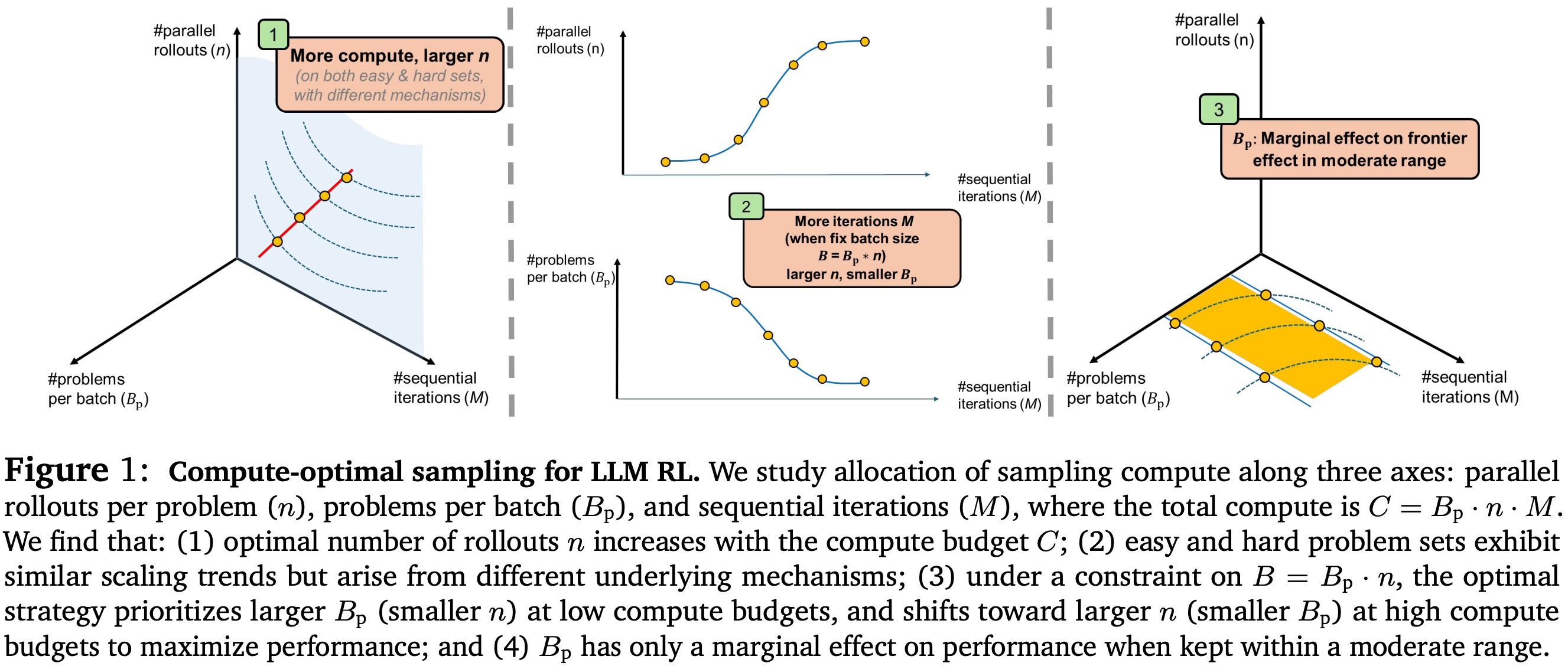
“We study the compute-optimal allocation of sampling compute for on-policy RL methods in LLMs, framing scaling as a compute-constrained optimization over three resources: parallel rollouts per problem, number of problems per batch, and number of update steps.” - from [3]

Sampling compute. The relationship between compute and performance is less straightforward in RL relative to pretraining. For both pretraining and RL, the training process involves a sequence of training—or model update—steps. At each pretraining step, a single forward and backward pass is performed. On the other hand, an RL training step includes multiple components:

• Data collection: sampling completions from the current policy.

• Optimization: updating the policy over collected data.

With this in mind, we can model the total compute cost of an RL training run as C = B_p​ × n × M, where B_p is the number of unique prompts per batch, n is the number of rollouts generated per prompt, and M is the number of steps taken during RL training. The analysis in [3] primarily focuses on compute spent on sampling completions (B_p and n) rather than sequential training steps (M).

Scaling laws for sampling. Given the compute footprint for RL outlined above, our goal is to better understand how varying the allocation of a fixed compute budget C_0 across the three factors B_p, n, and M impacts model performance. The scaling analysis is conducted in [3] by sweeping over settings of B_p ∈ {2^5, 2^6, …, 2^10} and n ∈ {2^3, 2^4, …, 2^11}, where both of these parameters are uniformly sampled via grid search on a log scale. Due to hardware constraints, a maximum effective batch size (B_p​ × n ≤ B_max) is also enforced.

From a given (B_p, n) setting, we can perform a single RL training run to capture increasing settings of M throughout training. Following scaling law best practices, model performance is evaluated during training by measuring reward on an in-domain validation set. The evaluation results in a training run are sub-sampled to only include record-breaking points—defined as points in the reward curve that exceed all prior rewards—along the learning trajectory; see below. By considering only record-breaking points when modeling an RL training run, we fit our scaling law to the frontier of the reward trajectory for this run.

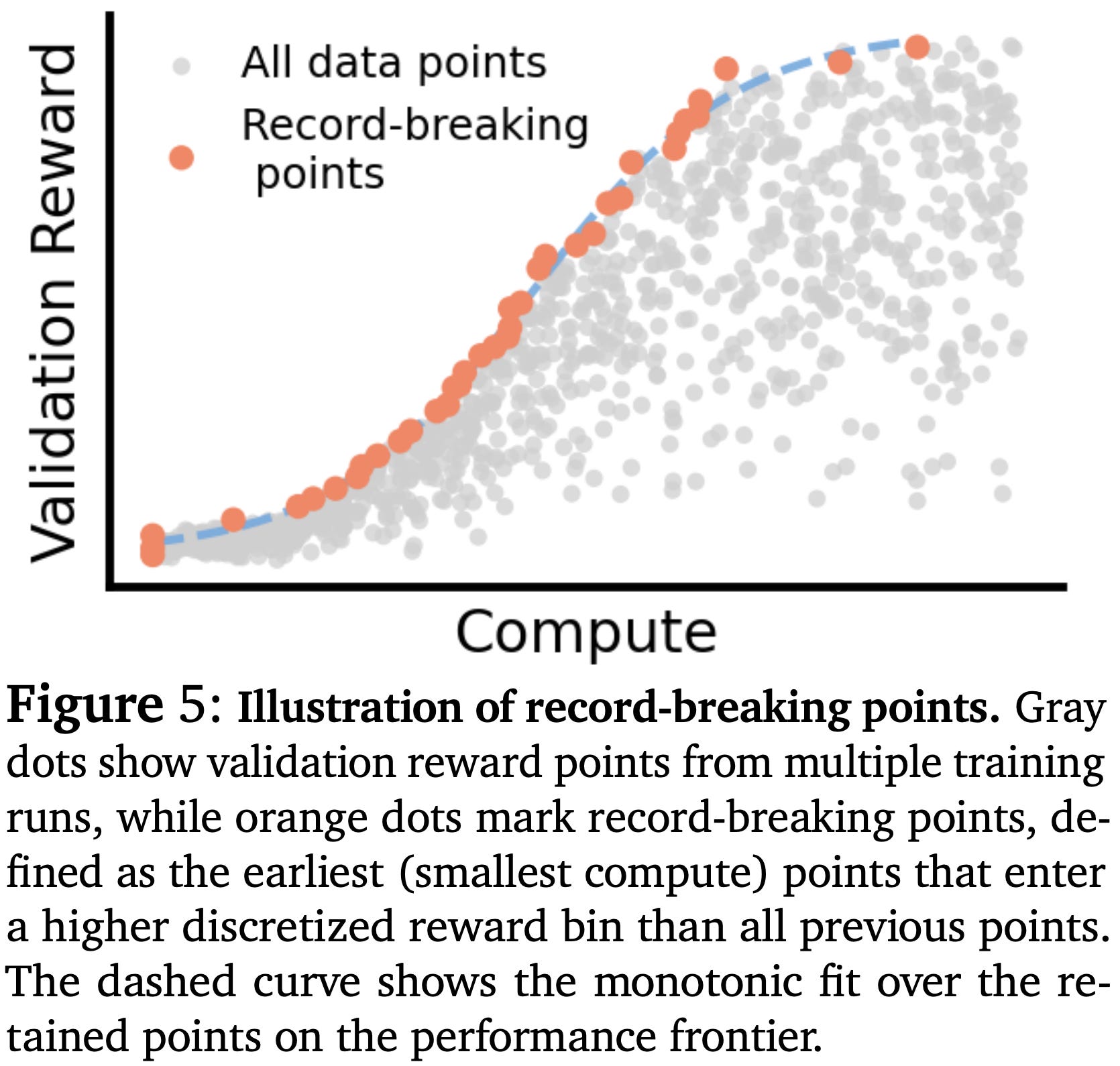
To robustly identify record-breaking points in the reward trajectory, rewards are separated into discrete bins, and the first point at which the reward enters a new bin is selected as the record-breaking point. Once the cleaned reward trajectory is available, we model this single training run with a sigmoidal scaling law—similar to the scaling law formulation used in [1]. This gives us a collection of scaling laws for RL training curves with different settings of B_p and n, allowing the optimal configuration to be identified at each compute level from run-specific curves.

Building on these run-specific scaling laws, we can also fit a scaling law on the optimal settings identified for each compute level. Namely, we can use a similar sigmoidal scaling law to model how the optimal value of n varies according to our compute budget C, allowing us to extrapolate optimal training settings at higher compute budgets. In theory, the same approach can be used for B_p, but no clear pattern is observed in practice for the optimal value of B_p.

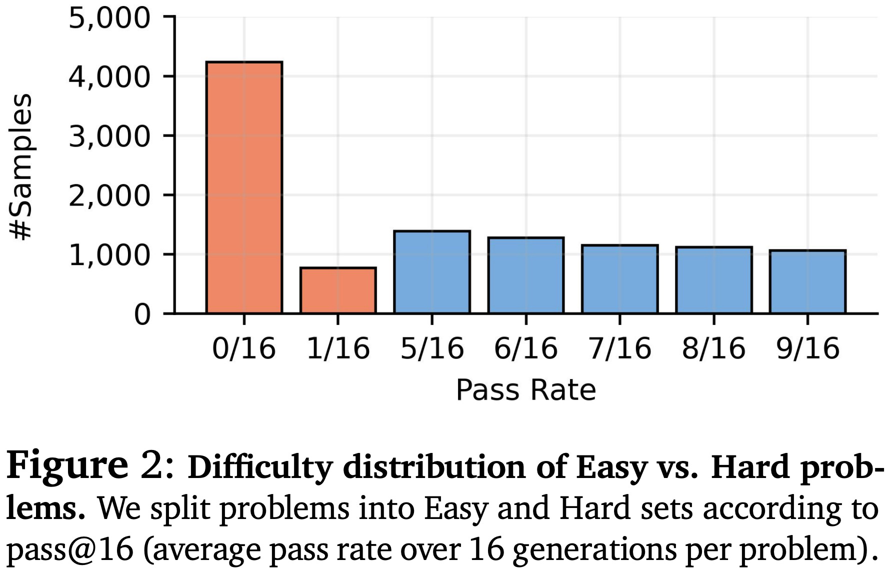
Experimental settings. The scaling analysis described above is conducted using Qwen2.5-7B-Instruct, Qwen3-4B-Instruct, and Llama3.1-8B-Instruct as base models. All RL training runs use binary outcome rewards and the vanilla GRPO optimizer. Guru-Math is used as the primary dataset and is split into easy and hard subsets by assessing the difficulty of each prompt—judged by the accuracy of the base model over 16 rollouts (i.e., Avg@16). The difficulty distribution is shown below with the easy and hard subsets shaded in blue and orange, respectively. Empirical scaling analysis is performed separately on both easy and hard data subsets in [3] to observe how difficulty distributions impact trends in scaling.

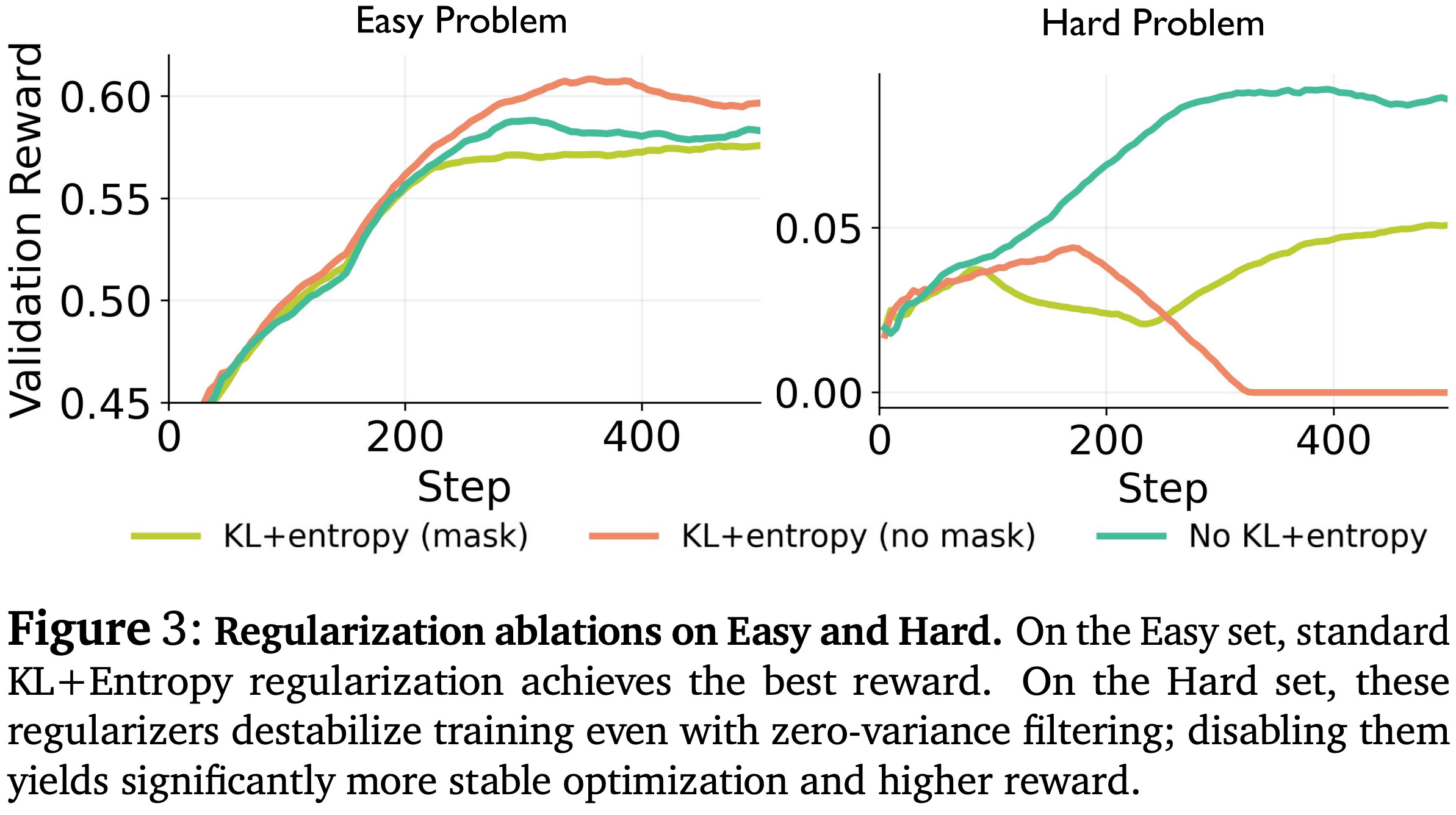
In order to make the RL training process stable, the correct regularization strategy is needed. Interestingly, we see in [3] that optimal regularization is difficulty-dependent. Authors consider adding both a KL divergence and entropy bonus to the RL training objective. On easy problems, the entropy bonus helps to prevent premature entropy collapse in the policy. However, using an entropy bonus on difficult problems can actually cause an entropy explosion by pushing the policy towards rare but successful reasoning trajectories, making it better to remove regularization entirely. As shown below, the following regularization strategy is found to yield the most stable results8:

• Apply both the entropy bonus and KL divergence—which helps to delay entropy explosion—in tandem when training on the easy dataset.

• Use no regularization when training on the hard dataset.

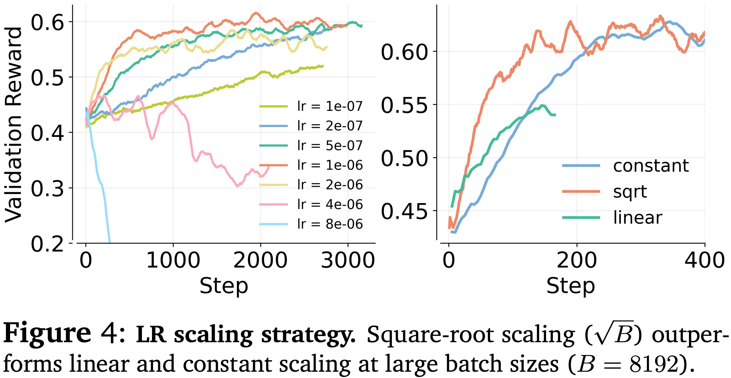
In addition to difficulty-dependent regularization, the learning rate must be increased with the batch size to ensure stable training. In particular, a square root scaling rule is used for the learning rate in [3], which increases the learning rate proportionally to the square root of the batch size; see below.

How should we allocate compute? The primary takeaway from the scaling analysis in [3] focuses upon the number of rollouts to sample (n) for each prompt in a batch. As the compute budget increases, the optimal setting of n increases as well, eventually saturating at higher compute budgets; see below. In other words, allocating increased compute towards sampling more rollouts per prompt yields better results compared to just training the model for longer. Interestingly, the exact scaling law also depends on the problem difficulty—smaller optimal values of n are observed when training on a harder dataset.

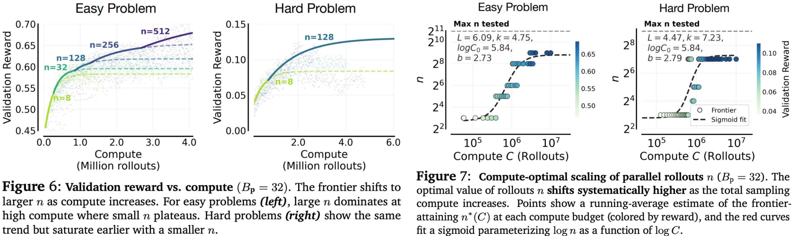
This trend holds for all base models across both easy and hard training datasets. Intuitively, scaling n has a different impact depending on the problem difficulty:

• Sampling more rollouts on easy problems can sharpen performance (i.e., improve Avg@K) for problems that are already solvable and improve policy robustness by lowering the probability of an incorrect rollout.

• Increasing the number of rollouts increases exploration and, in turn, aids in discovering rare solutions to difficult problems in order to improve the ratio of problems that can be solved (i.e., Pass@K) by the policy.

Interestingly, B_p has only a moderate performance impact when kept within a reasonable range and is found to primarily influence training stability.

Although the optimal setting of n scales with increasing compute, the exact shape of this scaling law—and the point at which it saturates—changes depending on the exact training setup. Therefore, while the scaling trends hold across different settings, the exact scaling parameters must be fit to the particular RL training setup being used. Practically, authors in [3] recommend the following approach for determining an optimal compute allocation in RL:

1. Execute RL training runs at lower compute budgets by varying the value of B_p and n but restricting the value of M.

2. Fit a scaling law, using the approach described above, from these results.

3. Infer the optimal value of n from the scaling law.

4. Choose the minimum value of B_p that yields stable training.

5. Invest the remaining compute budget into additional training steps M.

This approach provides us with a predictable process for extrapolating the optimal compute allocation for RL from lower-budget experiments.

We now have a detailed understanding of scaling laws for both pretraining and RL. However, one of the primary takeaways from this overview is the fact that a “scaling law” is completely different between these two domains. To close, we will briefly discuss the key ways that scaling laws differ between pretraining and RL, explain why these differences exist, and outline key takeaways from research on RL scaling that remain useful despite the overall messiness of RL.

Measuring performance. Pretraining scaling laws predict a particular metric: the cross entropy loss (or another related entropy metric) measured over an in-domain, held-out validation set. This performance metric is stable and is typically computed over a large, diverse dataset (i.e., a random sample of the pretraining corpus). Such a stable, diverse, and specific metric provides the perfect y-axis for fitting a scaling law and allows us to clearly define the impact of specific design decisions on the resulting model. RL scaling laws make an attempt to retain this robustness; e.g., performance is computed over an in-domain validation set. However, RL scaling laws typically use the reward (or accuracy) of the policy9 as the underlying metric to which scaling laws are fit. This is a downstream performance metric that can fluctuate substantially depending on the domain being studied, the benchmark being used, and the composition of data in that benchmark. As a result, scaling laws for RL tend to be more noisy and domain specific relative to those used for pretraining, which capture a more general trend in model performance.

Defining compute. Pretraining has a very clean compute footprint that is usually estimated with the number of training FLOPs C = 6 × N × D. This clean definition of compute provides an obvious x-axis for our scaling law. In contrast, RL compute is difficult to define due to the presence of both sampling and policy updates. The exact definition of compute used in RL scaling laws may change depending on the paper we are reading. For example, some papers derive a FLOP-like metric similarly to pretraining [3], while others rely on the number of GPU hours used [1]. Either way, the wall-clock time of RL training varies substantially depending on the framework being used, which means that the relationship between GPU hours and raw compute is not consistent. These factors must be considered when fitting a scaling law for RL because they cause the details of scaling laws to change depending on the exact setup being used.

Practical takeaways. Despite the fact that RL scaling laws tend to be messy and bespoke, there are still several useful trends that we can learn from the papers in this overview:

• The scaling behavior of RL is predictable within a given setup. Intra-model extrapolation works well and can be used to judge the viability of your setup during the early training phases. Inter-model extrapolation is also effective and can yield useful insights, though these insights may not always transfer across different training configurations.

• The impact of design decisions on RL is not singular. Some decisions impact learning efficiency, while others impact asymptotic model performance. This distinction is important because degradations in efficiency can be solved by simply training for longer, while a degradation in asymptotic performance may not be trivially recoverable. Interestingly, many recent GRPO variants seem to primarily benefit learning efficiency and stability [1].

• Using larger models yields consistently positive results in the RL scaling laws we have seen, though the presence of compute constraints can create interesting tradeoffs. When training with less data or compute, we may actually benefit from using a smaller model due to the fact that learning efficiency saturates with model size.

• To invest more compute into RL, we can i) run training for more steps or ii) use more inference compute at each step. Interestingly, even though the compute cost of RL is dominated by inference, most scaling laws suggest that allocating more compute to sampling completions is helpful. RL training is surprisingly robust to data reuse, benefits from large batch sizes, and scales predictably as we sample more completions per prompt in a batch.

Hi! I’m Cameron R. Wolfe, Deep Learning Ph.D. and Staff Research Scientist at Netflix. This is the Deep (Learning) Focus newsletter, where I help readers better understand important topics in AI research. The newsletter will always be free and open to read. If you like the newsletter, please subscribe, consider a paid subscription, share it, or follow me on X and LinkedIn!

[1] Khatri, Devvrit, et al. “The art of scaling reinforcement learning compute for llms.” arXiv preprint arXiv:2510.13786 (2025).

[2] Tan, Zelin, et al. “Scaling behaviors of llm reinforcement learning post-training: An empirical study in mathematical reasoning.” arXiv preprint arXiv:2509.25300 (2025).

[3] Cheng, Zhoujun, et al. “IsoCompute Playbook: Optimally Scaling Sampling Compute for LLM RL.” arXiv preprint arXiv:2603.12151 (2026).

[4] Shao, Zhihong, et al. “Deepseekmath: Pushing the limits of mathematical reasoning in open language models.” arXiv preprint arXiv:2402.03300 (2024).

[5] Zheng, Chujie, et al. “Group sequence policy optimization.” arXiv preprint arXiv:2507.18071 (2025).

[6] Yu, Qiying, et al. “Dapo: An open-source llm reinforcement learning system at scale, 2025.” URL https://arxiv. org/abs/2503.14476 1 (2025): 2.

[7] Liu, Zichen, et al. “Understanding r1-zero-like training: A critical perspective.” arXiv preprint arXiv:2503.20783 (2025).

[8] Chen, Aili, et al. “Minimax-m1: Scaling test-time compute efficiently with lightning attention.” arXiv preprint arXiv:2506.13585 (2025).

[9] F. Yao, L. Liu, D. Zhang, C. Dong, J. Shang, and J. Gao. Your efficient rl framework secretly brings you off-policy rl training, Aug. 2025. URL https://fengyao.notion.site/off-policy-rl.

[10] Chen, Aili, et al. “Minimax-m1: Scaling test-time compute efficiently with lightning attention.” arXiv preprint arXiv:2506.13585 (2025).

[11] Piché, Alexandre, et al. “Pipelinerl: Faster on-policy reinforcement learning for long sequence generation.” arXiv preprint arXiv:2509.19128 (2025).

[12] Shao, Zhihong, et al. “Deepseekmath: Pushing the limits of mathematical reasoning in open language models.” arXiv preprint arXiv:2402.03300 (2024).

[13] Kaplan, Jared, et al. “Scaling laws for neural language models.” arXiv preprint arXiv:2001.08361 (2020).

[14] Hoffmann, Jordan, et al. “Training compute-optimal large language models.” arXiv preprint arXiv:2203.15556 10 (2022).

[15] Guo, Daya, et al. “Deepseek-r1: Incentivizing reasoning capability in llms via reinforcement learning.” arXiv preprint arXiv:2501.12948 (2025).