Olmo 3 and the Open LLM Renaissance

As the capabilities of large language models (LLMs) have continued to progress, AI research has generally become less accessible to those outside of frontier labs. Although a variety of open-source LLMs are publicly available, there are two key issues that have consistently impeded progress in open research:

• The performance gap between closed and open models.

• The prevalence of open-weight models, and the scarcity of fully-open models.

Put simply, most “open” LLMs only publicly release the model’s weights (and sometimes an accompanying technical report). However, these weights are only a shallow snapshot of the model’s training process. To reproduce any component of this training process, more artifacts (e.g., data, code, training recipes, and deeper technical details) are needed. The limitations of open-weights LLMs have caused fully-open LLMs to become more popular, with AI2’s Open Language Model (Olmo) series being one of the most prominent proposals in the space. In this post, we will provide a comprehensive and understandable overview of Olmo 3 [1]—the most recent release in the Olmo series and top-performing fully-open LLM.

“We introduce Olmo 3, a family of state-of-the-art, fully open language models at the 7B and 32B parameter scales. The release includes… every stage, checkpoint, datapoint, and dependency used to build [Olmo 3]. Our flagship model, Olmo 3 Think-32B, is the strongest fully open thinking model released to-date.” - from [1]

As we will see, Olmo 3 lags behind the performance of top frontier models, but the value of these models lies in their transparency. In addition to providing a detailed technical report [1], Olmo 3 releases model checkpoints across the entire training process, all of the training data, and full training and evaluation code—the models can be completely retrained from scratch using these resources. For these reasons, the value of Olmo 3 goes beyond simply providing better, fully-open LLMs. For anyone interested in contributing to open LLM research, Olmo 3 and its artifacts are among the most comprehensive starting points to ever be released.

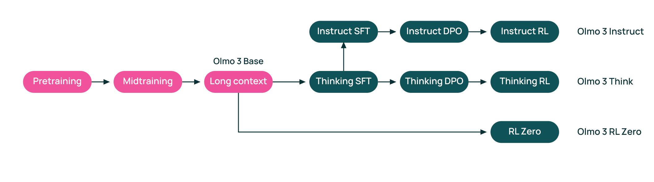
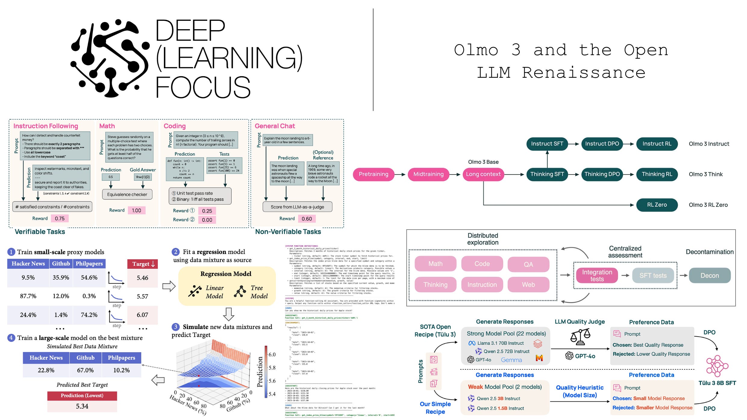
Model flow. The high-level training pipelines, referred to as “model flows” in [1], used for training both sizes (i.e., 7B and 32B) of Olmo 3 models are shown above. Base models for Olmo 3, which are also openly released, are created via a three-stage process of general pretraining, midtraining on targeted data, and a context extension phase. From here, base models undergo a sequential post-training process that includes supervised finetuning (SFT), direct preference optimization (DPO), and RL training to produce multiple Olmo 3 model variants:

• Olmo 3 Instruct: non-reasoning models that quickly respond to user queries and are optimized for multi-turn chat, instruction following, and tool usage.

• Olmo 3 Think: reasoning models that undergo specialized training to hone their complex reasoning capabilities by outputting long chains of thought (or reasoning trajectories) prior to providing a final answer.

• Olmo 3 RL-Zero: reasoning models that are created by running reinforcement learning (RL) training directly on the pretrained base model—this setup was popularized by the DeepSeek-R1 model [9].

Notably, the training algorithms and pipeline used for the Instruct and Think models are quite similar, but the data are modified to target unique capabilities. After covering necessary details of the Olmo 3 model architecture, we will explain in detail each component of this training process—beginning with pretraining and ending with reasoning-oriented RL training—in an end-to-end fashion.

Preliminaries. This overview outlines the entire training pipeline for Olmo 3. In a single overview, we cannot cover all necessary background information needed to understand how a near-frontier-level LLM is trained. Instead, most important concepts will be explained inline as they are introduced throughout the overview. Additionally, an index of important topics that will appear throughout the overview (with links for further learning) is provided below:

• LLM pretraining and scaling laws.

• Supervised Finetuning (SFT) and Direct Preference Optimization (DPO).

• Reasoning models.

• Reinforcement Learning with Verifiable Rewards (RLVR).

• Group Relative Policy Optimization (GRPO).

“The goal of Olmo 3 Base is to establish a strong foundation that supports a diversity of general capabilities while enabling downstream capabilities like thinking, tool-use, and instruction-following to be easily elicited during post-training.” - from [1]

A new base model is pretrained from scratch for Olmo 3 with a special focus on key capabilities like reasoning and agents (i.e., function calling or tool use). These capabilities are usually elicited during later post-training stages, but we lay the groundwork during pretraining by exposing the model to a diverse dataset and building a robust knowledge base. Specifically, Olmo 3 undergoes three separate phases of pretraining:

1. A general pretraining stage over a large textual corpus.

2. A midtraining phase focusing on targeted, high-quality data.

3. A context extension phase teaching the model to handle longer inputs.

To improve upon Olmo 2 [3], authors in [1] explore new data curation strategies and iterate on the pretraining process in a scientifically rigorous manner. An expanded suite of benchmarks and evaluations that meaningfully capture base model performance across diverse experimental settings is also created, allowing the highest-performing pretraining recipe to be discovered empirically.

Training infrastructure. Pretraining code and recipes for Olmo 3 are available in the Olmo-Core repository, allowing all Olmo 3 model checkpoints to be exactly reproduced. The pretraining process relies upon Fully-Sharded Data Parallel (FSDP)1 distributed training, which saves memory by sharding2 parameters, gradients, and optimizer states across GPUs; see below. During the forward and backward passes, each GPU gathers the full parameters for the current layer from the shards distributed across all GPUs, computes the necessary operations, and then re-shards the parameters—and gradients after the backward pass—before moving on to the next layer. As a result, we only store a single full layer in GPU memory at any given time, while all other layers are sharded across GPUs.

FSDP is also performing data parallel training (i.e., the “DP” part of FSDP). In addition to sharding, each GPU processes a unique mini-batch of data, allowing the total batch size to reach 8× (assuming eight GPUs) the maximum batch size of a single GPU. For example, we can see the full training settings for the Olmo 3 32B Base model below, which uses a total batch size of 1,024 during pretraining. Given that the pretraining process uses 1,024 GPUs in total, this means that each GPU in the cluster is processing a single sequence during a training step.

When pretraining a modern LLM like Olmo 3, we use more than just a single eight-GPU node. For example, we just mentioned that Olmo 3 is pretrained with 1,024 H100 GPUs (or 128 eight-GPU nodes), while midtraining and long context training use 128 and 256 GPUs, respectively. However, sharding across thousands of GPUs is inefficient because inter-node communication is much slower than intra-node communication. To solve this, we usually apply FSDP inside of each eight-GPU node and create replicas of the model across nodes to avoid constantly communicating model parameters—which is very expensive—between nodes.

“We ran on 128 nodes with 8× NVIDIA H100 (80GB HBM3) per node, connected via TCPXO (200 Gbps/GPU). We used HSDP via PyTorch FSDP2 with 8-way sharding so each node hosted a single model replica. Communication-intensive collectives were therefore restricted to within-node, improving efficiency.” - from [1]

Within each node, FSDP is used to shard the model, while across nodes, standard data parallelism is used. Each node has a full copy of the model, and gradients are averaged across nodes at each step. This way, we sync parameters and gradients across nodes during each model update, rather than performing syncs at every layer as in FSDP. This approach, called Hybrid-Sharded Data Parallel (HSDP), is used during all phases of training for the Olmo 3 Base models.

The primary limitation of the HSDP setup described above is the fact that it does not shard everything. For example, full activations are stored on each GPU! When performing long context training, storing the full activations on each GPU can lead to memory issues. As a solution, authors in [1] add Context Parallelism (CP) to their distributed training setup, which splits the model’s input across multiple GPUs in a node along the sequence dimension to reduce memory overhead; see above. To support a multi-node setup, we can apply CP in tandem with FSDP inside of a node, then create data parallel replicas across nodes as in HSDP.

Base model evaluation. The performance of Olmo 3 Base models across a wide variety of benchmarks is presented in the table below. Among fully-open models—meaning weights, data, and code are all available—like Marin 32B and Apertus 70B, Olmo 3 Base models achieve state-of-the-art performance and make notable gains in the math and coding domains. When including open-weights models like Qwen and Gemma, Olmo 3 performs comparably in some domains (e.g., question answering), while lagging behind in others (e.g., math and code).

When analyzing the performance of Olmo 3 models, we will notice that they are not usually state-of-the-art when compared to open-weights LLMs. However, Olmo 3 models do outperform fully open models and approach the performance of the best open-weight models in most domains. Because the Olmo 3 model series discloses its full training dataset, certain data sources must be removed from training to retain a commercial license. Open-weight models, due to not disclosing training data, do not operate under this restriction, which may (partially) explain the gap in performance. Despite lagging slightly behind the state-of-the-art, however, Olmo 3 models are an invaluable contribution due to their transparency and the ecosystem of tools they provide for further research.

The model architecture used by Olmo 3 [1] (shown above) is a dense3, decoder-only transformer architecture very similar to that of Olmo 2 [3]. There are two model sizes released—7B and 32B parameters—which have the same structure, differing only in the following aspects:

• Number of self-attention heads.

• Number of key and value heads (in self-attention).

• Dimension of hidden layers and token vectors.

• Number of total layers.

This architecture follows most design decisions found in other popular open LLMs, such as the Qwen-3 [21] series. Notably, Olmo 3 maintains the post-normalization structure (with RMSNorm) that was shown by Olmo 2 to improve training stability. Additionally, QK-norm is used, meaning an additional RMSNorm layer is applied to queries and keys before computing the attention operation. This additional normalization avoids attention logits from becoming too large, which can aid in training stability (especially for low precision training). This same approach is also used by models such as Gemma-3 and Olmo 2.

In the 7B model, attention layers in Olmo 3 are regular, multi-headed attention layers instead of Grouped Query Attention (GQA) layers. In contrast, the 32B model uses GQA with 40 attention heads and only eight key and value heads. As shown below, GQA shares keys and values—but not queries!—between multiple attention heads, which benefits both parameter and compute efficiency.

However, the biggest benefit of grouped-query attention comes at inference time. Memory bandwidth usage during inference is reduced because fewer keys and values need to be retrieved from the model’s KV cache. Given that memory bandwidth is the key bottleneck for the decode step during the transformer’s inference process, this change drastically speeds up the inference process.

To further improve attention efficiency, Olmo 3 uses Sliding Window Attention (SWA), which only considers tokens inside of a sliding window—Olmo 3 adopts a window size of 4K tokens is particular—during attention to save costs; see below. SWA is used in 3/4 layers—every fourth model layer uses full attention. SWA is a common architectural choice used by GPT-OSS, Mistral, Gemma and more.

Finally, Olmo 3 uses Sigmoid Linear Unit (SiLU) activations and is pretrained with a context window of 8K tokens. In a later training stage, Olmo 3 undergoes context extension using YaRN [8], which will be discussed more later in the overview. For a from-scratch implementation and detailed explanation of the Olmo 3 architecture, see this recent notebook from Sebastian Raschka, or his extensive architecture comparison that includes most open LLMs.

Developing a solid pretraining recipe is an empirical process—we need to test a bunch of settings and see what works well. Given that pretraining is expensive, the number of full-scale pretraining runs we can perform is limited. Instead, we test interventions to the pretraining process by:

1. Formulating smaller-scale tests to validate our ideas.

2. Applying promising interventions to full-scale runs.

However, such an approach can still be difficult—results at a small scale may not translate well to larger-scale experiments. Some benchmarks may only be sensitive at specific scales. For example, small-scale pretraining tends to yield models with random performance on math and code benchmarks, but other benchmarks may already be saturated even at smaller scales. Additionally, the LLM evaluation process is generally noisy, so small differences in results may not be meaningful.

“If something hurts performance at small scale, you can confidently rule it out for large scale. But if something works at small scale, you should still make sure you’ve trained on a reasonable number of tokens to conclude with high probability that these findings will extrapolate to larger scales. The longer you train and the closer the ablation models are to the final model, the better.” - from [2]

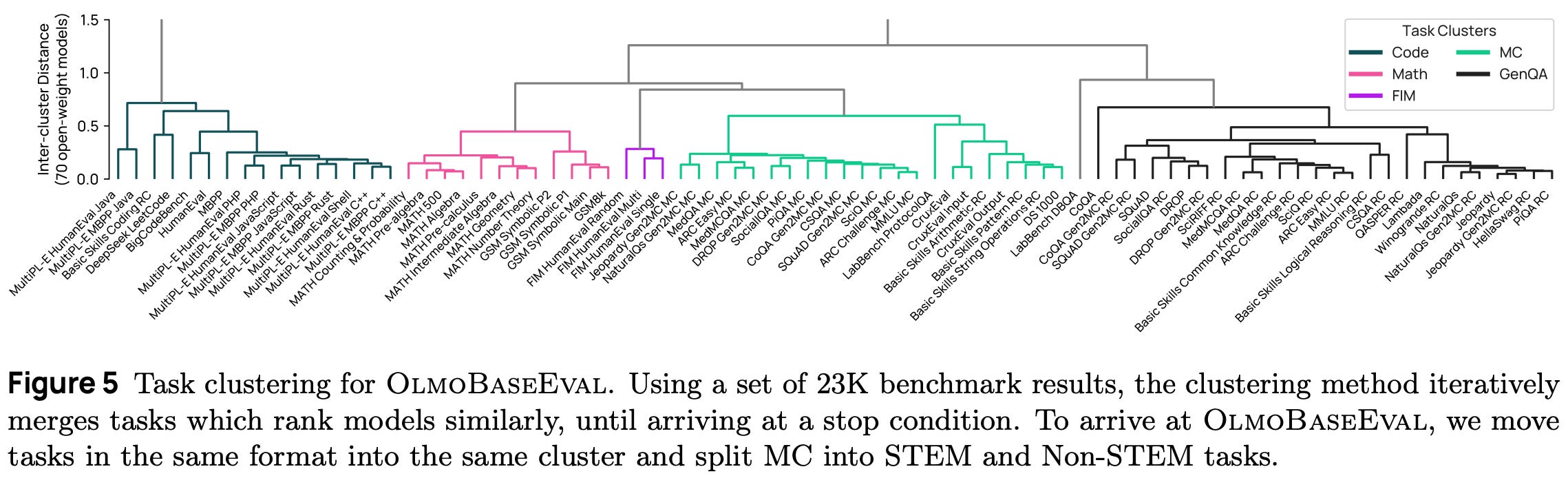
OlmoBaseEval is a set of 43 total benchmarks that is created to guide pretraining experiments for Olmo 3. This suite is 4× larger than the benchmarks used by Olmo 2. It covers a wide range of capabilities (including math and code), presents multiple newly proposed benchmarks, and maintains held-out test sets for several important capabilities targeted during pretraining. The benchmark is developed according to three major design principles:

1. Task Clusters: benchmarks are grouped into task clusters over which scores are aggregated, where each cluster targets a core capability.

2. Proxy Metrics: a detailed scaling analysis is performed to determine which tasks provide a useful signal at which scales.

3. Signal-to-Noise Ratio (SNR): benchmarks with high SNR4 are either removed from the evaluation suite or evaluated using a larger number of samples.

To form the task clusters, a pool of 23K benchmark scores is collected using 70 different open-weight models, then a clustering approach5 is used to group tasks with similar evaluation results together. In other words, a cluster includes tasks that tend to rank models similarly during evaluation. Some manual post-processing is performed to arrive at the final task clusters: multiple-choice (MC) STEM, MC non-stem, Math, Code, and Code Fill-in-the-Middle (FIM); see below.

A suite of 25 Olmo 2 [3] models trained with varying amounts of compute—and a few other open-weight base models—are used to conduct a scaling analysis, allowing us to observe the scale at which particular metrics become useful; see below.

Based on this analysis, evaluation tasks are separated into two groups:

• Base Easy: tasks that show signal at smaller scale.

• Base Main: tasks that were not yet saturated at larger scales.

The Base Easy task suite includes all tasks from Base Main that have ground truth answers available. Performance on this suite is measured in bits-per-byte6, which is computed by dividing the negative log-likelihood of the ground truth answer by the number of bytes in the answer string. Using bits-per-byte as a proxy metric for evaluating a pretrained LLM provides a less noisy measure of performance without requiring advanced instruction following capabilities. Other common strategies include perplexity-based evaluation or multiple choice questions.

“Continuous proxy metrics have been shown to be a better decision making tool for model performance before we exit the noise floor.” - from [1]

The OlmoBaseEval suite is used across pretraining and midtraining. The Base Easy suite is used as a proxy for evaluating smaller-scale pretraining runs, while full-scale pretraining and midtraining runs are evaluated with Base Main. The entire OlmoBaseEval suite is openly available in the Olmes repo from AI2 and can be run on any model, as shown below (taken from the Olmes README).

# Run the base easy evaluation (for evaluating small-scale experiments)
olmes \
    --model allenai/Olmo-3-1025-7B \
    --task \
        olmo3:base_easy:code_bpb \
        olmo3:base_easy:math_bpb \
        olmo3:base_easy:qa_rc \
        olmo3:base_easy:qa_bpb \
    --output-dir <output_dir>

# Run the base main evaluation
olmes \
    --model allenai/Olmo-3-1025-7B \
    --task \
        olmo3:base:stem_qa_mc \
        olmo3:base:nonstem_qa_mc \
        olmo3:base:gen \
        olmo3:base:math \
        olmo3:base:code \
        olmo3:base:code_fim \
    --output-dir <output_dir>

# Run the base held-out evaluation
olmes \
    --model allenai/Olmo-3-1025-7B \
    --task \
        olmo3:heldout \
    --output-dir <output_dir>

Evaluation during pretraining. When running pretraining, we usually want to monitor the intermediate performance of our model. However, the learning rate has a huge impact on evaluation results. To get meaningful metrics, we must anneal (or decrease according to a schedule) our learning rate to zero prior to this evaluation being performed—this simple approach is followed for the Olmo 3 7B model but is expensive. As an efficient alternative, authors in [1] adopt a model merging approach from [6] for their 32B model that merges four checkpoints that are 1,000 steps apart before performing evaluation. This approach has been found to accurately simulate learning rate annealing behavior during pretraining.

“We demonstrate that merging checkpoints trained with constant learning rates not only achieves significant performance improvements but also enables accurate prediction of annealing behavior. These improvements lead to both more efficient model development and significantly lower training costs.” - from [6]

Model merging combines multiple models with the same architecture by taking a linear combination of their weights. This approach might seem bizarre, but it works well because LLMs finetuned from the same pretrained model are mode connected—taking a linear combination of two such models’ weights produces another model that performs well. We can use model merging to combine multiple models into a hybrid model that shares the models’ capabilities. One of the simplest model merging approaches is a model soup [22], which simply averages the weights of multiple model checkpoints. We can find public implementations of various model merging techniques in MergeKit, which is also used in [1]. A full overview of model merging techniques can be found at the link below.

The pretraining process for Olmo 3—including both experiments and final training runs—consumes over 90% of total compute for the project and targets four key capabilities: science, medical, math and coding. Dolma 3 Mix, which contains 6T tokens derived from the full Dolma 3 pool of 9T tokens, is the primary data source used for pretraining and is created using the steps illustrated above. These steps mostly match other open pretraining recipes [2, 3, 4], aside from:

• Using token-constrained mixing and quality-aware upsampling (details to follow) to improve the overall quality of tokens included in the mixture.

• Including a new set of academic PDF data—238M unique PDFs in total with a knowledge cutoff of December 2024. This data is curated using a custom PDF crawler that prioritizes academic sites and paper repositories then converted into linear plain text with OlmOCR.

For Olmo 3 pretraining, authors only consider data sources that have a sufficient number of tokens to meaningfully impact model capabilities during pretraining—additional small but high-quality data sources are reserved for midtraining. Structured data (e.g., question-answer pairs or chat templated data) is also saved for midtraining. Including structured data in pretraining—even if the token quantity is small—significantly impacts evaluation results and can complicate data ablations.

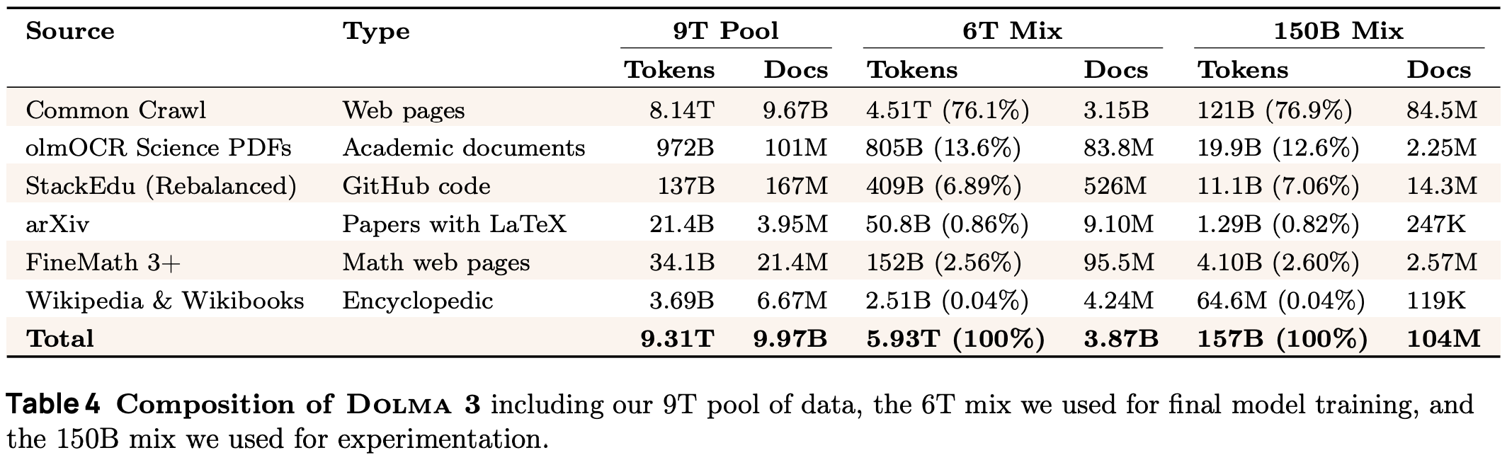
Mixing approach. The full Dolma 3 pool contains 9T tokens, but we must mix and sample this pool—under the constraint of the total number of tokens we want to use for training (i.e., 6T for Olmo 3)—to create the best possible pretraining corpus. As shown in the table above, Dolma 3 is partitioned into groups by type, and we must determine the optimal mixing ratio for each of these groups. The strategy for determining the best data mixture in [1] has two components:

1. A base procedure that constructs a high-quality data mix over a fixed (i.e., not being actively changed or developed) set of data sources.

2. A conditional mixing step that efficiently updates our existing mix as data sources change during the model development process.

“We apply a mixing strategy that draws on swarm-based methods to train and evaluate many smaller proxy models, using these results to inform an optimal mix. Further, we apply a novel conditional mixing procedure to account for the fact that our data sources were being constantly refined and updated.” - from [1]

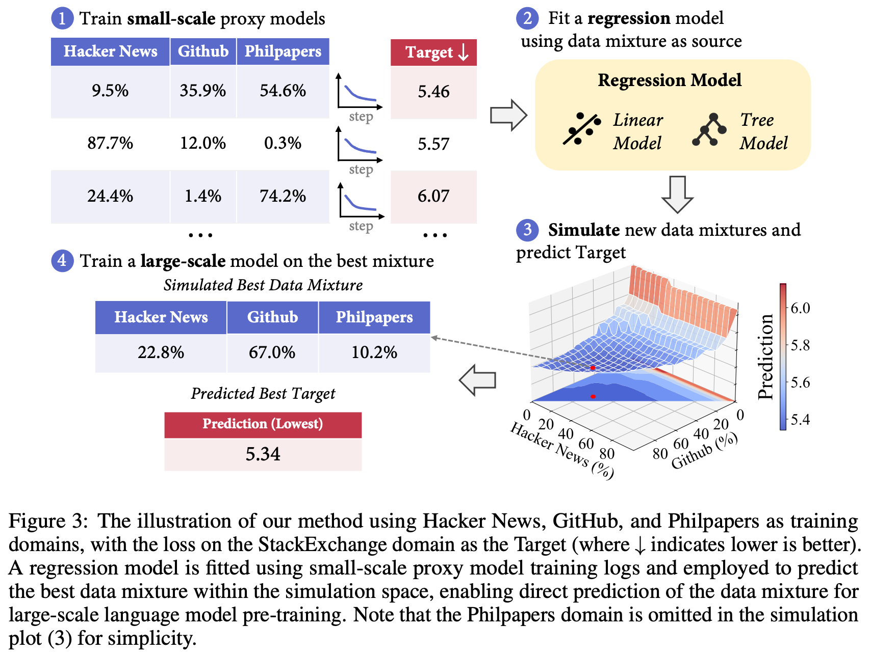
The base procedure in [1] uses a swarm optimization approach that is similar to the idea of RegMix [5]. The swarm optimization proceeds as follows:

1. Randomly sample a large number of mixtures. In [1], the number of mixtures sampled is set to 5× the number of data sources being mixed.

2. Perform small proxy experiments by training a 30M parameter Olmo 3 model over 3B tokens from each mixture.

3. Evaluate each proxy model on the Base Easy suite.

4. For each task in the Base Easy suite, train a generalized linear model that predicts task performance given the mixing parameters as input.

5. Use the generalized linear models to simulate performance of different data mixtures and search for the optimal data mixture under constraints.

In [1], authors have a maximum token budget and aim to not repeat any domain in the data more than four to seven times. These constraints are added to the final optimization step when searching for the optimal data mixture. From here, we can take the optimal data mixture and test it at a larger scale; see below.

During model development, we will usually search for the optimal data mixture more than once. Data sources are constantly changing and being improved, which influences the optimal mixture. Additionally, some sources of data may become available later in the development process. Re-running the base procedure from scratch is inefficient—not all sources of data are changing. Instead, a conditional mixing approach is proposed [1], which avoids re-computing the full swarm by:

• Beginning with a base mixture that has already been optimized.

• Treating this mixture as a “virtual” data source with frozen mixing ratios.

• Considering all new or modified data sources.

• Re-running the base procedure with both new and virtual domains.

Multiple rounds of data mixing are performed for Olmo 3, including an initial round to optimize the mixture of web data and several conditional mixing rounds that added code and PDF data to the mixture. Properties of the final data mixture are shown below7, where we can see that training on the optimal data mixture—as opposed to the natural data distribution—improves performance on most tasks.

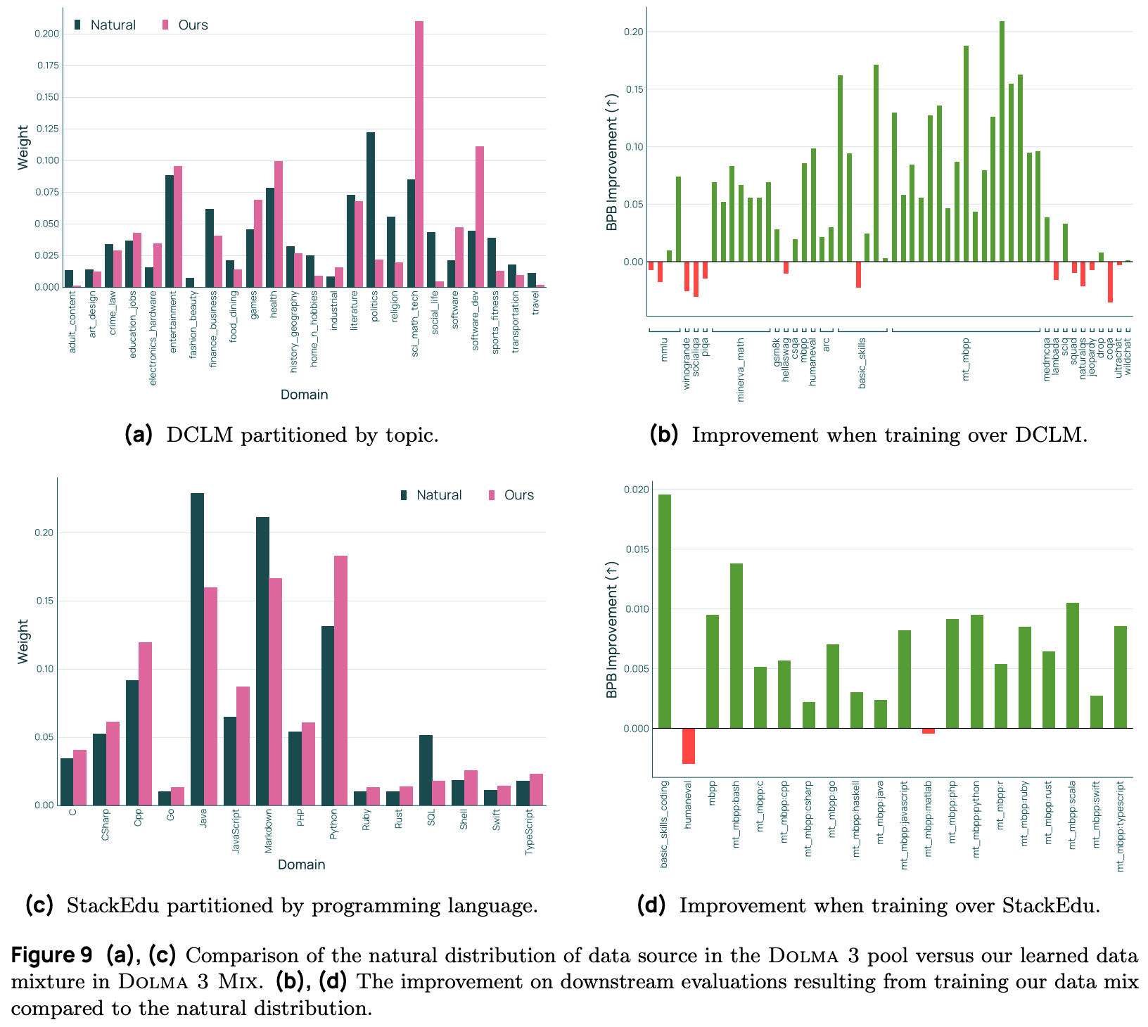
The mixing strategy described above is also flexible and can be used to optimize more than just domain mixtures. For example, when optimizing the code mixture in [1], authors fix the overall ratio of code data at 25% and instead optimize the mixture of programming languages within this hard-coded token budget.

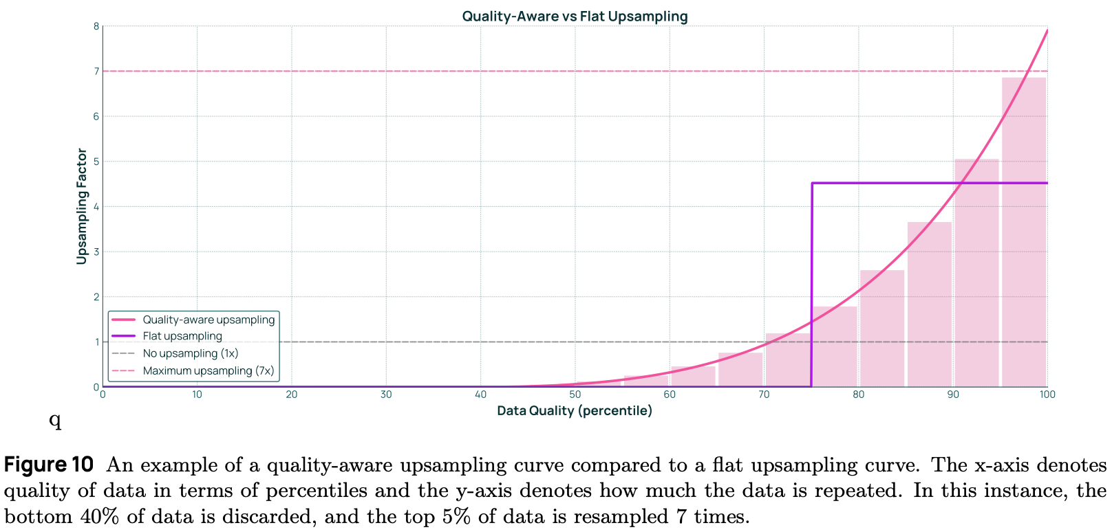
“We found that quality-aware upsampling improves performance in data-constrained settings… We achieved better results by upsampling the highest-quality data: including multiple copies of the top 5% and single copies of the remaining data to reach the target token count.” - from [1]

Quality-aware upsampling. We can further improve performance by upsampling—or including multiple copies of—the highest quality data in the training mixture. This effect can be achieved by first running all data through a quality classifier and forming an upsampling curve as shown below, where the x-axis represents data quality and the y-axis is the upsampling factor. If we were to filter data with a fixed quality threshold, this upsampling curve would be a step function, but authors in [1] model upsampling as a monotonically increasing curve. For example, we see below that the highest quality percentile of data receives an upsampling factor of ~7×, meaning the data is repeated seven times in training.

A separate upsampling curve is formed for every topic in the pretraining data. To find this curve, we start with our known constraints for pretraining:

• The optimal mixture of topics (i.e., determined by data mixing).

• The total number of desired tokens for training.

• The maximum upsampling factor.

From here, we can perform a search over the space of parametric curves to find one that meets these constraints. Once the curve is found, the data for a topic is separated into a discrete set of quality buckets or percentile ranges. We can compute the upsampling factor for a given bucket by integrating the upsampling curve over this bucket and dividing this integral by the width of the bucket.

Following the primary pretraining phase for Olmo 3, the model undergoes continued midtraining and long context training. The training objective during these phases is identical to that of pretraining, but we i) adopt more targeted datasets and ii) train for fewer tokens. For example, midtraining and long context training for Olmo 3 each train the model over an additional 100B tokens.

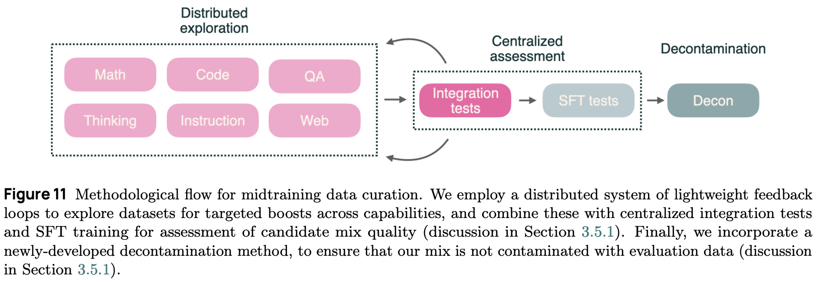
Midtraining for Olmo 3 uses the Dolma 3 Dolmino Mix, which contains 100B tokens curated to enhance key model capabilities. This data mix is derived via a two-part iterative process (illustrated above):

1. Parallel (or distributed) feedback: many data sources are considered in parallel via efficient microannealing experiments [2] that use lightweight training runs to ablate each data source8.

2. Integration tests: any data sources yielding promising microannealing results are combined into a centralized annealing run over a 100B token dataset that includes all promising sources of data at that time.

This approach creates a distributed feedback loop that allows many sources of data to be efficiently explored and brings promising data sources together for centralized integration tests. Put simply, we can repeatedly vet data sources in parallel and validate them at larger scales until we arrive at the final mixtraining mix. Five rounds of integration tests were performed when developing Olmo 3.

“This methodology allowed us to make rapid, targeted assessments of the quality of datasets being considered for the midtraining mix, and to iterate on many data domains in parallel.” - from [1]

To evaluate models during midtraining, authors rely primarily upon the Base Main dataset, which consists of benchmarks that are not yet saturated during pretraining. Additionally, lightweight SFT experiments are performed with midtrained models to test the “post-trainability” of various data mixtures. The performance of Olmo 3 models on these benchmarks after iterative rounds of microannealing experiments and integration testing is outlined below.

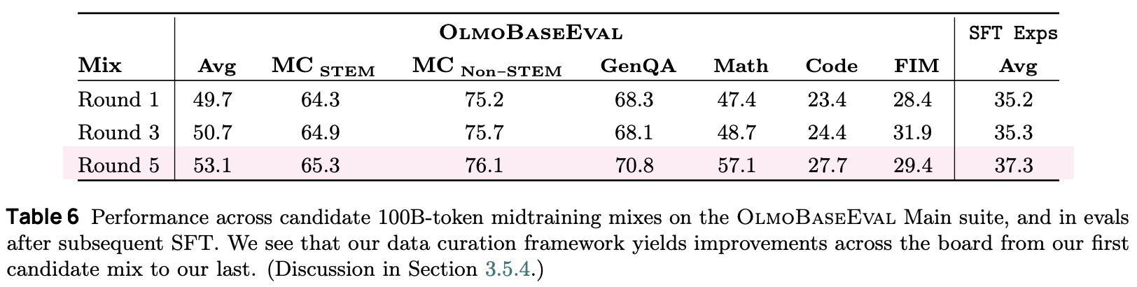
The final midtraining mix includes some pretraining data to avoid model drift. Additionally, instruction and thinking (or reasoning) data is included, which is found to benefit performance almost universally across benchmarks and helps to lay early groundwork for post-training. All instruction and reasoning data avoids using templates or special tokens during midtraining due to the complexity that this additional formatting introduces into the evaluation process. Instead, text formatting is adopted, which maintains the pretrained model’s output format.

“Although individual sources and domains present performance tradeoffs, the inclusion of these cross-domain post-training data types in aggregate is consistently beneficial, and this benefit begins even before post-training.” - from [1]

We observe very clear domain tradeoffs during midtraining. For example, math and code performance can be improved by increasing the ratio of this data in the midtraining mixture, but such improved performance comes at the cost of degraded performance in other domains. The Dolma 3 Dolmino mix strikes a balance between important domains. Interestingly, the final midtraining model is also a merge of two independently-trained models with different seeds, which authors find to improve performance compared to using an individual model.

Long context9 training is an important component of modern LLMs that plays a huge role in real-world tasks (e.g., tool usage or multi-turn chat) and helps with enabling test-time scaling for reasoning models. However, pretraining an LLM from scratch with natively long context would be incredibly expensive—long sequences consume a lot of memory and compute during training. To get around this, most LLMs are pretrained using much shorter sequences (e.g., 8K tokens in the case of Olmo 3) and undergo a context extension phase after pretraining.

“Because training with long sequence lengths is computationally costly, most language models are pretrained with shorter sequences and extended only in a later stage of model development. During the extension phase, models are trained on longer documents, and positional embedding hyperparameters are typically adjusted to ease positional generalization.” - from [1]

The details of this context extension phase vary drastically between models. For example, the number of tokens used for long context training can be anywhere between 100B (or less) to 1T tokens, and the order of training phases changes between models—the long context phase could be placed before midtraining or even included as part of post-training. Olmo 3 adopts a straightforward pipeline that performs long context extension after midtraining and before post-training. This long context phase uses a 100B token mix10 of the full 600B token Dolma 3 Longmino pool to extend the context of Olmo 3 from 8K to ~65K tokens.

Long context data. The dataset for long context training includes a combination synthetic data and long documents sourced from the academic PDF pretraining corpus. This data undergoes heuristic GZIP filtering that removes any document in the top and bottom 20% of GZIP compressibility. In other words, we remove long context documents that are the least or most redundant. Interestingly, this GZIP heuristic outperforms more sophisticated, model-based techniques that use perplexity metrics to identify documents with long-range token dependencies.

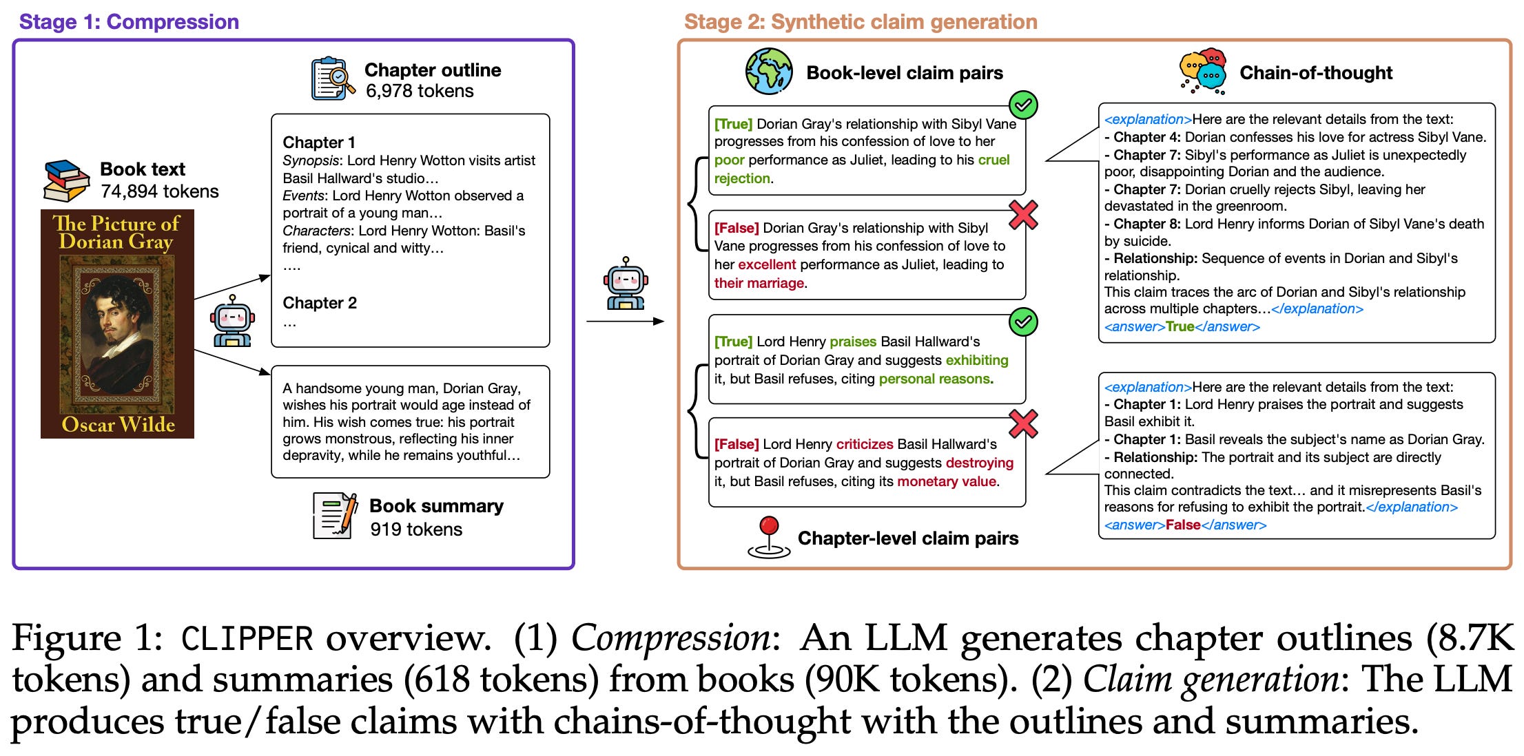
Beyond PDF data, authors in [1] collect synthetic long context data that is focused on information extraction tasks over long documents. Specifically, the technique used to generate long context data is inspired by CLIPPER [7]; see above. This approach avoids making the assumption that the LLM being used to generate synthetic data already has long context abilities. Instead, we do the following:

1. Partition a long document into several sections.

2. Identify the most common noun phrases in each section11.

3. Extract (k=8) text snippets from the section for each noun phrase.

4. Provide this information in a prompt to an LLM—Olmo 2 32B is used in [1]—to synthesize an aggregation task; e.g., writing a summary, providing a list of true or false claims, creating a conversational explainer, and many more.

We can then train our model to replicate these synthetic outputs using only the long document as input, which teaches the model to reliably extract information. During long context training, this data—including both the PDF and synthetic data—is mixed with short context data from midtraining at a 1:2 ratio (i.e., 34% long context and 66% short context data) to form the Dolma 3 Longmino Mix.

Data during long context training varies drastically in terms of sequence length. Naively batching sequences together would yield excessive padding. When we batch sequences together, we create a fixed-size tensor of size B (batch size) × S (sequence length) × d (embedding dimension). Here, S is either the maximum context length during training or the size of the longest sequence in our batch. Usually, each sequence is shorter than S, and we occupy the rest of this tensor with padding tokens to maintain the fixed shape needed by the GPU.

In the case of long context training, most examples will have length ≪S—most of this tensor will be occupied by empty padding tokens that waste computation; see above. To solve this issue, we can use document packing, which batches sequences together in the same row to avoid excessive padding; see above. Additionally, we add an inter-document mask to the attention process to avoid attention across examples that are packed together. This approach is used by Olmo 3 to improve the efficiency of the long context training process; see here for more details.

“We experiment with several methods for extending RoPE… including adjusted base frequency scaling, position interpolation, and YaRN. Each approach is applied either to all RoPE instances or is restricted to RoPE used in full attention layers. We find that applying YaRN only to full attention layers yields the best overall performance” - from [1]

Context Extension. Several different context extension techniques are tested in [1], and YarN [7] is found to yield the best performance on key evaluations like advanced Needle-in-a-Haystack (NIH) tests, RULER, and HELMET. Full details on YarN and other context extension techniques can be found in this overview.

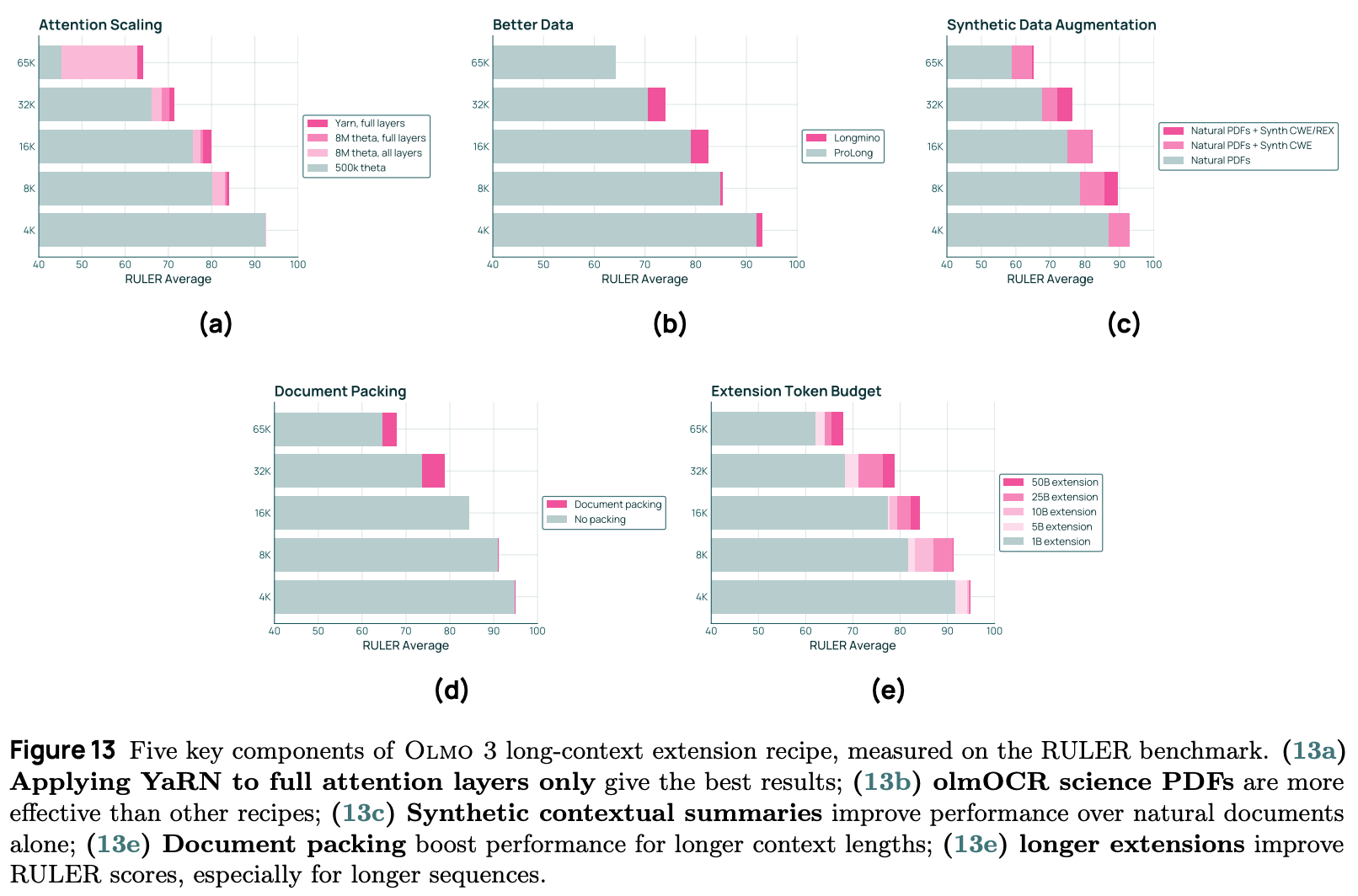
YaRN is only applied to full attention layers, while positional embeddings are left unchanged in layers that use SWA. As shown in the figures above, this extension approach, when combined with an increasing amount of curated long context data, significantly benefits the long context performance of Olmo 3 models.

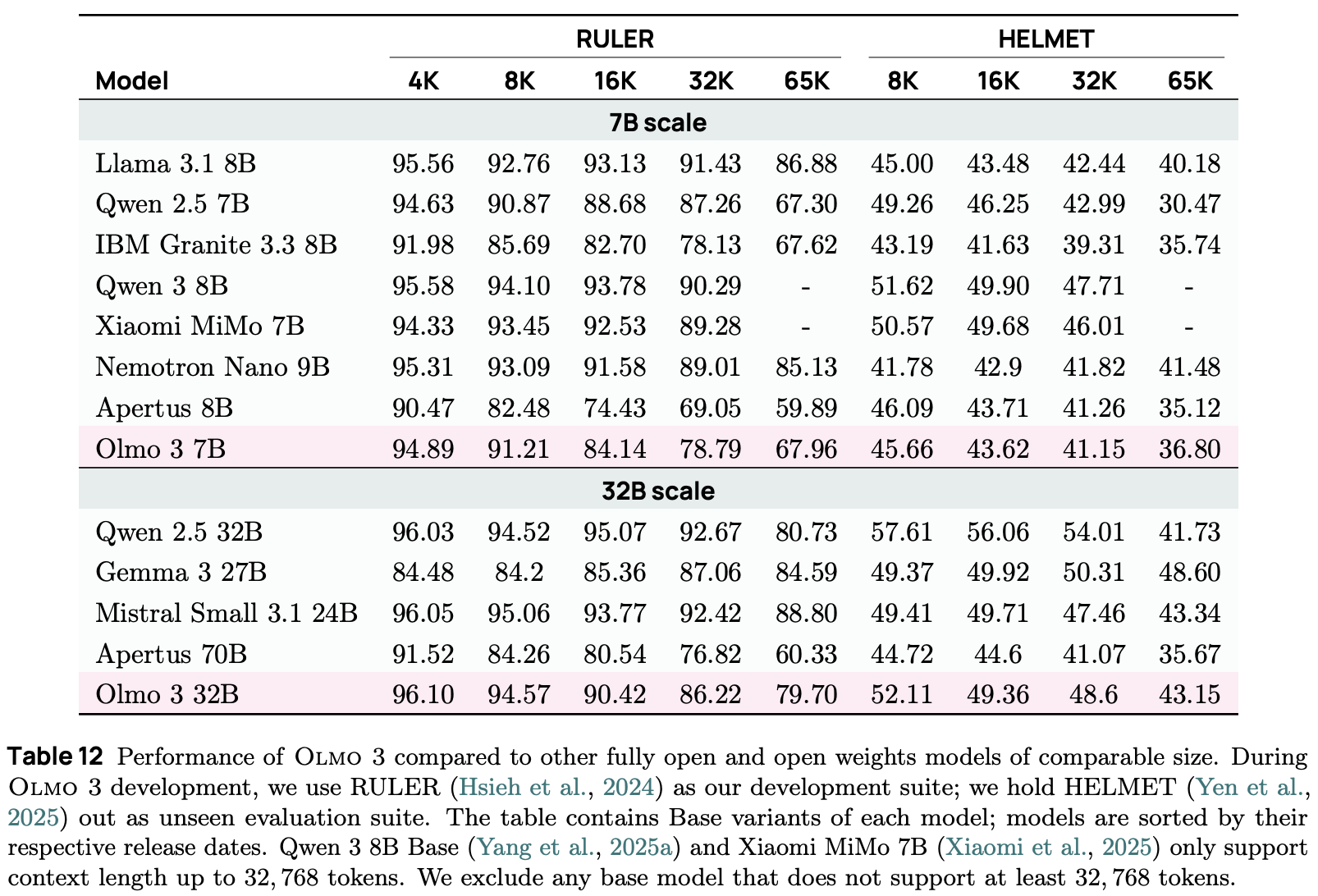
Model merging continues to play a role in long context training, but we cannot run multiple long context training runs with different seeds due to the high cost of long context training. Instead, authors in [1] take three (adjacent) checkpoints from the end of a single long context training run and merge them, which further benefits performance. The long context capabilities of Olmo 3 are comparable to or slightly worse than that of the Qwen-2.5 models, as shown in the table below.

“Olmo 3 Think is trained for reasoning by generating extended thoughts before producing a final answer. To achieve this, we curate high-quality reasoning data (Dolci Think), apply a three-stage training recipe (SFT, DPO, and RLVR), and introduce OlmoRL infrastructure, which brings algorithmic and engineering advances in reinforcement learning with verifiable rewards.” - from [1]

Expanding upon the Olmo 3 Base models, authors in [1] explore post-training strategies to create a suite of reasoning models, referred to as Olmo 3 Think. These models are trained to reason by outputting long reasoning traces or trajectories prior to their final output via large-scale RLVR. For an in-depth overview of LLM-based reasoning models, please see the link below.

The reasoning training process for Olmo 3 Think models differs from other work in two keys respects:

1. Models are trained with both SFT and DPO prior to RLVR.

2. A multi-objective RLVR approach is used that mixes data from both verifiable and non-verifiable domains.

Despite differing slightly from related work, this post-training pipeline is shown in [1] to yield consistent gains across all stages (i.e., SFT, DPO, and RLVR).

Evaluation results. Relative to Olmo 2 [2], Olmo 3 Think models are evaluated over a much wider set of benchmarks that capture capabilities like math, general reasoning, knowledge, coding, instruction following, question answering, chat, and more. At the 32B scale, Olmo 3 Think models achieve state-of-the-art metrics among other fully-open thinking models, as well as match the performance of some popular open-weight models like Qwen-2.5 and Gemma-3; see below.

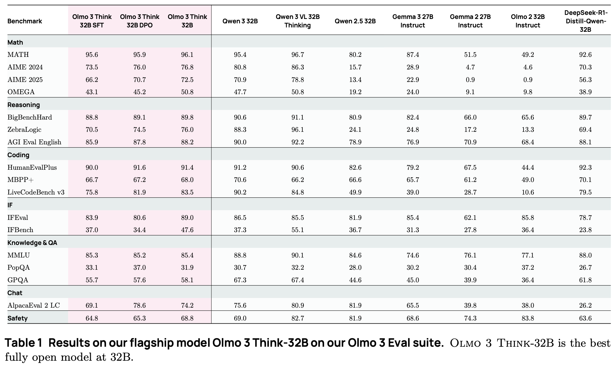
Compared to top open-weight reasoning models like Qwen-3, Olmo 3 Think narrows the gap in performance but is still lags behind. This gap is especially pronounced for 7B-scale models, where we see that Olmo 3 Think is significantly outperformed by Qwen 3 on knowledge-based tasks (e.g., MMLU). Such results align with general trends in performance for Olmo 3—these models are close to state-of-the-art and provide many benefits in terms of transparency and openness.

Prior to RL training, we finetune the base model using both SFT and DPO in order to create a more useful starting point for RL. The purpose of these training stages is to both improve capabilities and, more specifically, teach the model to produce thinking traces prior to its final answer. We are seeding the model with the correct output format before performing RL. Notably, recent work on LLM post-training typically does not use all of these stages. For example, DeepSeek-R1 [9] either performs a lightweight SFT stage before RLVR or applies RLVR directly to the base model (i.e., an RL-Zero setup). We see in [1] that consistent gains can be realized by performing SFT and DPO prior to RL given proper data curation.

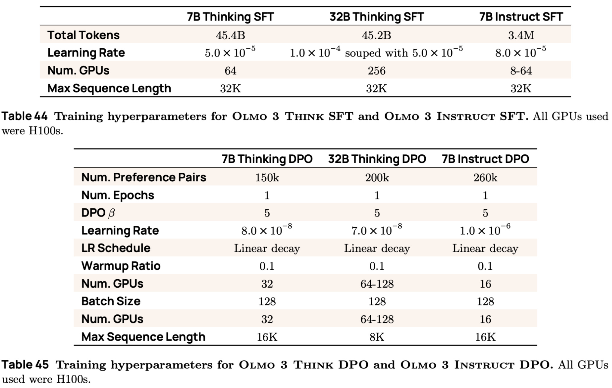
The key training settings for the SFT and DPO training processes performed with Olmo 3 are provided in the tables shown below for reference. The training code is present in Olmo-Core (for SFT) and OpenInstruct (for DPO).

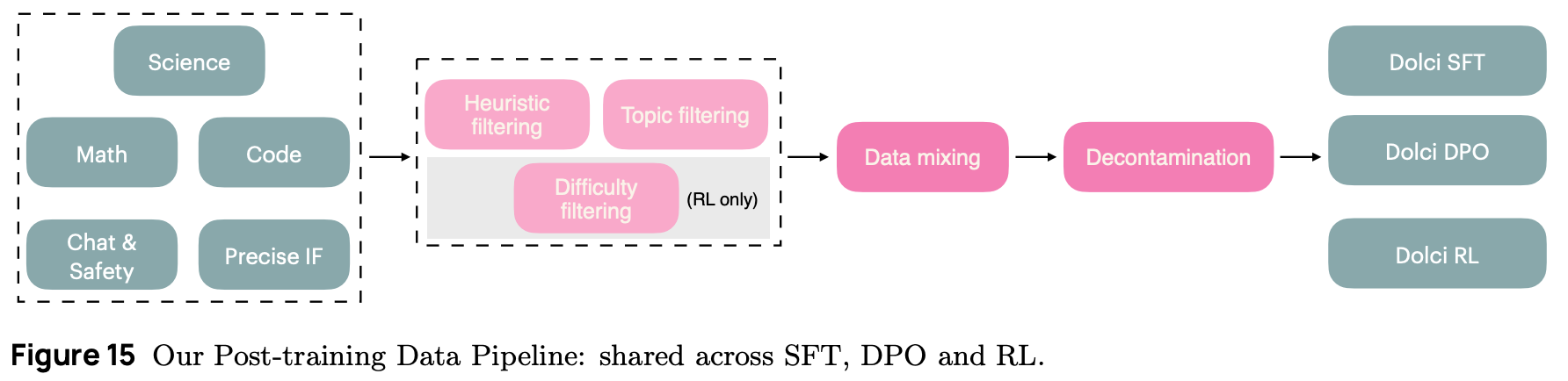
SFT. Dolci Think SFT is a set of ~2.3M supervised training examples that is used for the SFT stage of Olmo 3 and spans several important capabilities like math, science, coding, instruction following, chat and safety. This data is curated as follows (see above for a step-by-step illustration):

• Prompt sourcing: prompts are sourced for each capability from a wide variety of public datasets12.

• Re-generating examples: for prompts with incomplete completions, we generate new completion(s)—including both a reasoning trace and final answer for each completion—using either DeepSeek-R1 or QwQ-32B.

• Correctness filtering: completions are verified using various domain-specific strategies (e.g., synthetically-generated test cases for code or verifiers for specific precise instruction following constraints).

• Heuristic filtering: prompts are removed based on having unclear usage licenses, incomplete reasoning traces, excessive repetition, mention of other model providers, and other heuristics.

• Topic filtering: prompts are classified by topic according to the OpenAI query taxonomy, and any topics that are irrelevant to Olmo 3 (e.g., requests for image generation) are either filtered or downsampled.

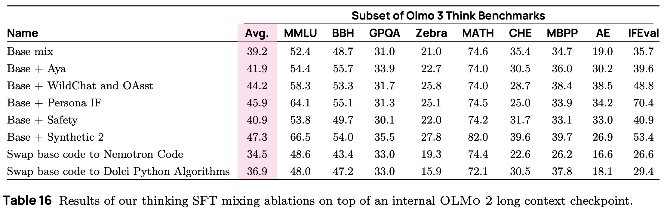
This post-training data curation process is generic and goes beyond SFT—a similar pipeline is used to curate data for DPO and RLVR. After prompts are sourced and filtered, the data mixture is derived using an approach very similar to that of midtraining: many data sources are gathered in parallel and tested via lightweight SFT experiments that train an LLM over 100B tokens from the domain of interest combined with an 100B token SFT base mixture. After evaluating data sources in parallel, we can perform centralized integration tests with data sources that are found to meaningfully benefit performance. Interestingly, all data sources in [1] were found to benefit performance on at least one evaluation benchmark; see below.

Beyond the post-training benchmarks used for Olmo 3, authors in [1] emphasize the role of “vibe checks”—or the manual inspection of a diverse (but usually small) set of model outputs by researchers—in evaluating models. Evaluation metrics and benchmark scores are useful, but they rarely tell the full story. By manually inspecting model outputs, we can discover trends in performance across experiments and training stages that might be difficult to uncover otherwise.

“Using [Olmo-Core], we can train a 7B model at 7700 tokens per second per GPU and a 32B at 1900 tokens per second per GPU… by relying on PyTorch’s built-in torch.compile(), custom kernels for operations such as attention and language modeling head, asynchronous and batched gathering of metrics, and asynchronous writing of checkpoints.” - from [1]

Similarly to pretraining and midtraining, the SFT training process uses the Olmo-Core codebase, which provides optimized code for supervised training. Compared to prior SFT training code for Olmo (i.e., found here in OpenInstruct), Olmo-Core is ~8× faster. Two epochs of training are conducted over Dolci Think SFT, and we again derive the final model via model merging. Specifically, we linearly merge the weights of two model checkpoints trained with different learning rates over the same data, forming the Olmo 3 7B and 32B Think SFT models.

DPO. Preference tuning is typically used for improving the alignment of an LLM to human preferences. In recent research on reasoning models, preference tuning is rarely used, but we see in [1] that DPO-based preference tuning yields an improvement in capabilities when used in tandem with SFT prior to the RL training phase. More specifically, Olmo 3 undergoes DPO-based preference tuning using a strategy that is inspired by Delta Learning [11]; see below.

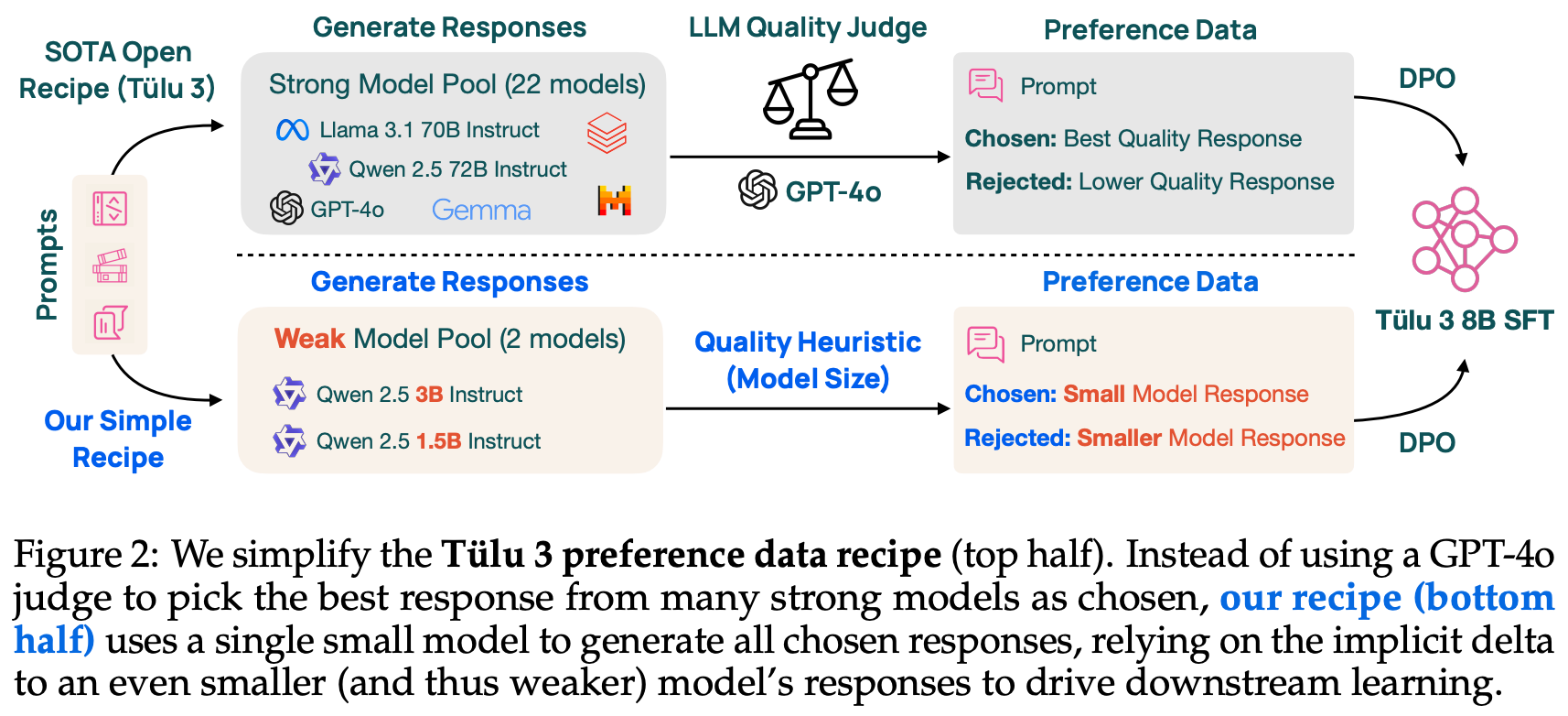
To create a preference dataset for DPO, prior models like Olmo 2 [3] leverage a synthetic data pipeline similar to UltraFeedback [20] that generates completions from a diverse pool of models. For each prompt, we do the following:

• Generate completions with each model.

• Rate each completion with an LLM judge.

• Form preference pairs based on these ratings (i.e., higher-scoring responses are preferred in a preference pair).

This approach hinges upon the diversity of the underlying model pool to yield high-quality preference pairs. Applying a similar model pooling approach in the reasoning domain would be difficult, as the number of LLMs with open reasoning traces is limited—most (proprietary) reasoning models surface only final outputs and hide their reasoning process. Delta Learning uses an alternative approach of forming high-quality preference pairs by minimizing the quality of rejected completions.

This approach focuses less on the absolute quality of completions in a preference pair and more on the relative quality difference between the chosen and rejected completions. For example, authors in [1] show that further training the Olmo 3 Think SFT model on synthetic completions from Qwen-3-32B actually degrades performance. However, we can improve Olmo 3 Think SFT performance via DPO with preference pairs that contain i) a chosen completion from Qwen-3-32B and ii) a rejected completion from the weaker Qwen-3-0.6B model.

“The intuition behind delta learning is that the quality of preference data depends primarily on the quality of the delta between chosen and rejected responses; the quality of either response individually is less important.” - from [1]

Olmo 3 Think DPO models are trained on Dolci Think DPO, a preference dataset comprised of completions with clear capability deltas that are generated using Delta Learning. As described above, model size is adopted as a simple heuristic for completion quality—chosen completions are sampled from the 32B Qwen model, while rejection completions are sampled from the 0.6B model. While all Olmo 3 Think SFT models are trained on a similarly-sized dataset, 7B and 32B Olmo 3 Think DPO models use preference datasets with 150K and 200K pairs, respectively.

Prompts for Dolci Think DPO are mostly reused from SFT, but additional sources of preference data from Olmo 2 (e.g., UltraFeedback and DaringAnteater) are also added. The same filtering operations from SFT are used by DPO, but filtering is only applied to chosen completions—rejected completions are left unfiltered. Due to the computational expense of experiments with reasoning traces, a hierarchical approach is used for finding the best data mixture. First, a wide variety of mixing experiments are performed using standard LLMs that directly provide output with no reasoning. The top three data mixtures from this phrase are then used in full reasoning experiments to find the best-performing preference mix.

As a final touch, Olmo 3 Think models undergo RL training using a combination of verifiable and non-verifiable rewards to improve the models’ reasoning skills while maintaining their general utility. The RL training process focuses upon the domains of math, code, instruction following, and general chat.

“We introduce OlmoRL, which includes our algorithm and closely intertwined engineering infrastructure to address challenges for RL with long reasoning traces, extending RLVR to include a wider variety of verifiable tasks.” - from [1]

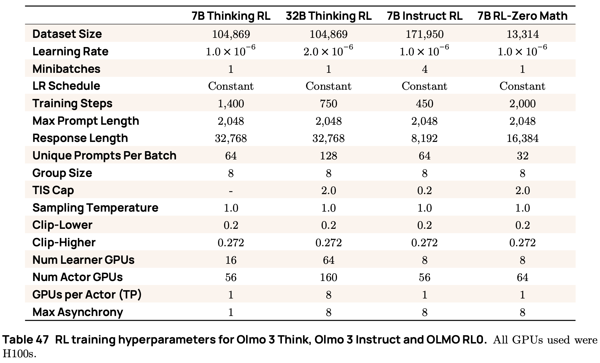
Detailed training configurations for each of the RL training processes performed using Olmo 3 are provided in the table shown below.

Reward signals. Most recent work on RL for reasoning models considers a pure RLVR setup with only verifiable rewards. For example, many works apply RL in math or coding domains [15, 17], where we can easily check the correctness of the model’s output via rules or test cases. In [1], the standard RLVR setup is extended to include rewards from both deterministic verifiers and LLM judges; see below.

The math domain uses a standard verifier that performs basic normalization of answers and equivalence checks via sympy to yield a binary correctness score. For coding and instruction following, correctness is checked via either test cases or constraint-specific verification functions. The reward in these domains can be binary (i.e., all tests must pass to receive a reward) or the ratio of tests that pass.

The general chat domain is not verifiable—we must rely upon an LLM judge to derive a reward. Authors in [1] use Qwen-3-32B as their judge model with thinking mode turned off and the prompt shown below. Depending on if ground truth outputs are available, the judge can either be reference-based or reference-free.

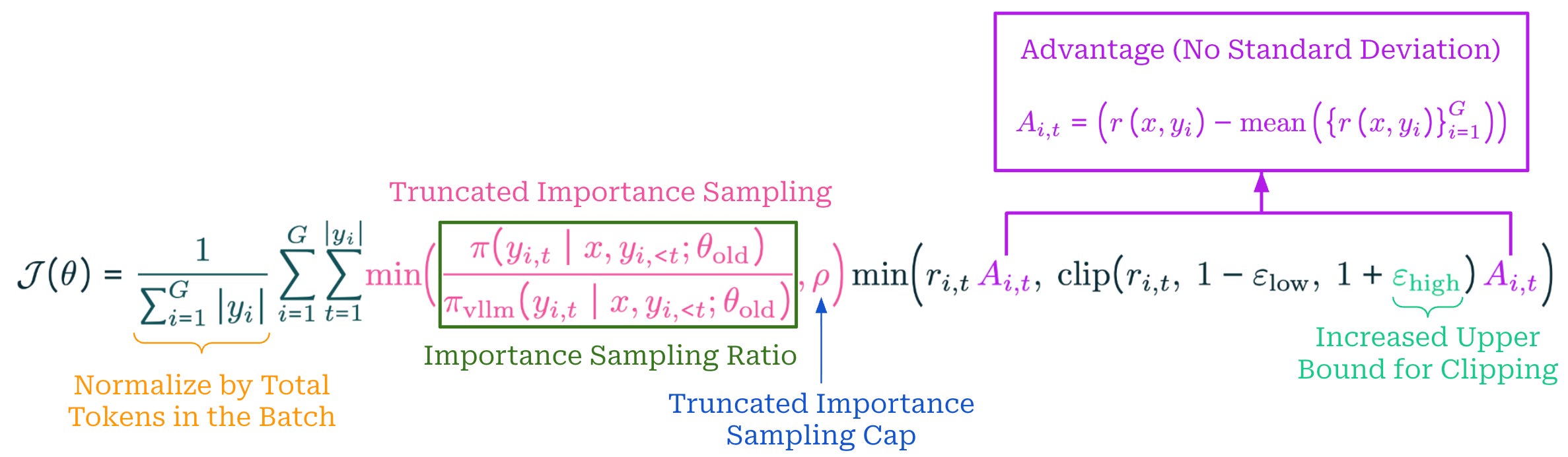
Enhancements to GRPO. Olmo 3 Think uses Group Relative Policy Optimization (GRPO) as the underlying optimizer for RL training. Inspired by a swath of recent papers that propose useful modifications to GRPO, authors in [1] adopt a wide set of improvements to the vanilla GRPO algorithm. The following enhancements are used in particular:

• Zero Gradient Filtering: prompts for which the entire group of completions or rollouts in GRPO receive the same reward are removed [16].

• Active Sampling: despite filtering zero gradient examples, a constant batch size is maintained by ensuring additional samples are always available to replace those that get filtered [16].

• Token-Level Loss: the GRPO loss is normalized by the total number of tokens across the batch instead of per-sequence, which avoids instilling a length bias in the loss [16].

• No KL Loss: the KL divergence term is removed from the GRPO loss to allow for more flexibility in the policy updates, which is a common choice in recent reasoning research [16, 17, 18].

• Clipping Upper Bound: the upper-bound term in the PPO-style clipping used by GRPO is set to a higher value than the lower bound to enable larger policy updates [16].

• Truncated Importance Sampling (TIS): an extra importance sampling term is added to the GRPO loss to adjust for differences in log probabilities between engines used for training and inference [18].

• No Standard Deviation: the standard deviation of rewards in a group is excluded from the denominator of the GRPO advantage calculation [19].

When considering all of these enhancements, the GRPO objective function is formulated as shown below. This objective maintains the structure of the GRPO objective, which is nearly identical to the objective from PPO but uses a modified advantage formulation. Compared to vanilla GRPO, however, we normalize the objective differently, slightly change the advantage, tweak the upper bound for clipping, and weight the objective using a capped importance sampling ratio.

More details on TIS. During RL training, we are constantly alternating between two key operations:

1. Rollouts: given a set of prompts, sample multiple completions to each prompt using the current LLM (or policy).

2. Policy Updates: computing an weight update for our LLM using the sampled rollouts and the objective function outlined above.

To improve efficiency, these operations are usually handled by separate engines. We sample rollouts using an optimized inference engine like vLLM or SGLang and compute policy updates with training frameworks like transformers—or usually a distributed version of this framework that uses an algorithm like FSDP or ZeRO. The use of different backends for rollouts and policy updates can lead to a mismatch between the two environments in which the log probabilities for a rollout differ significantly from those used in the policy update; see below.

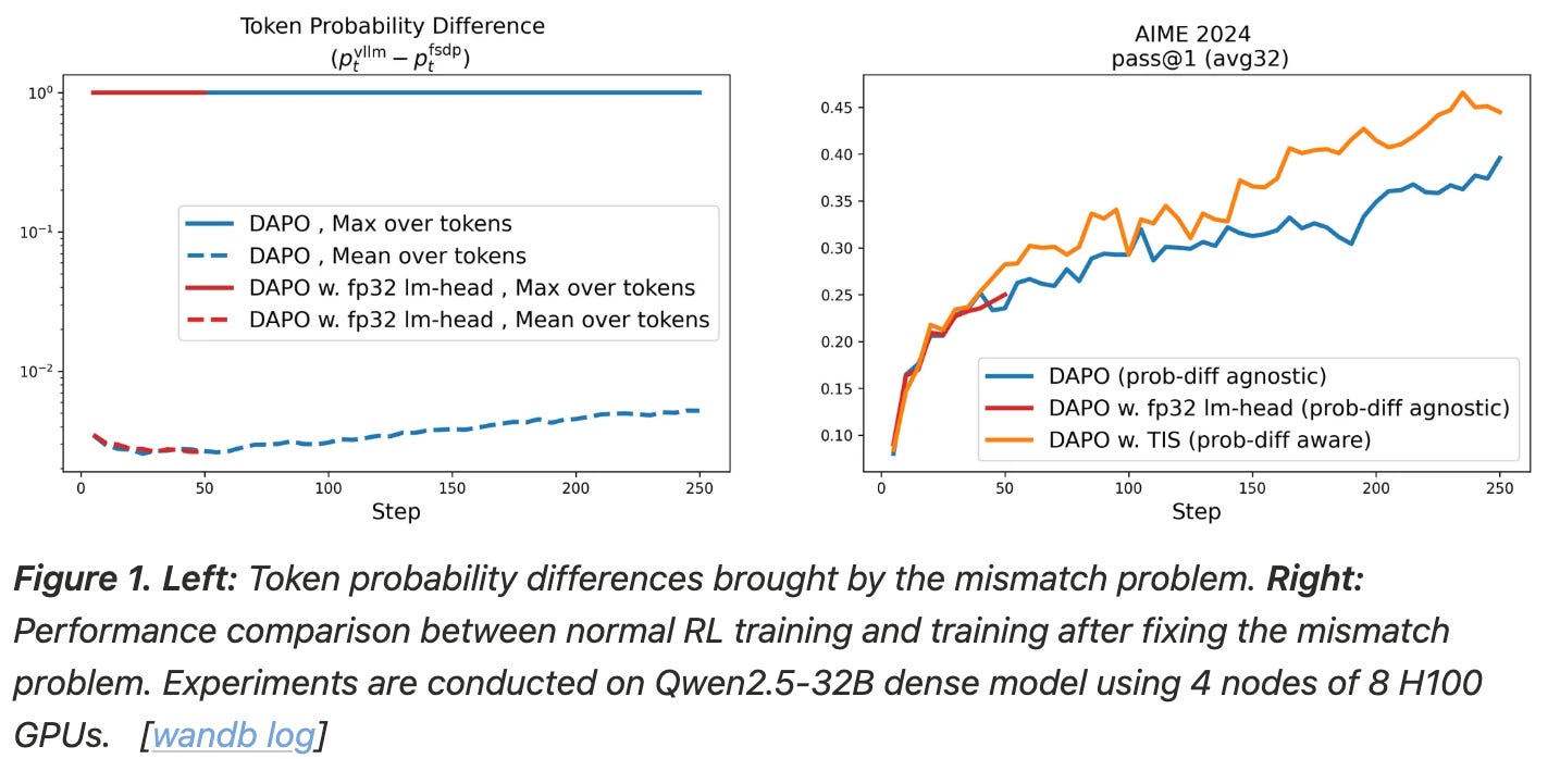
This mismatch persists even when steps are taken to reduce differences between inference and training backends. As a solution, authors in [18] use a truncated importance sampling scheme that re-weights the GRPO objective by the ratio of log probabilities from the two engines. We cap (or truncate) this importance sampling ratio at a maximum value of ρ. Without this correction, the RL training process becomes slightly off-policy, which can degrade performance. Using TIS re-weights examples with significant mismatches to solve this issue; see below.

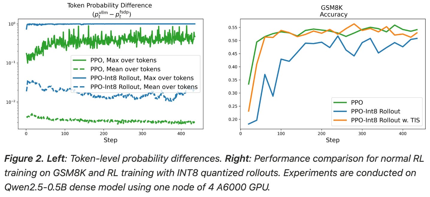
“This importance sampling term seems to be essential to getting modern RL infrastructure right, as without it, scaling to more complex systems is hard to get numerical stability with…. the advantage or reward is getting re-weighted by an importance sampling log-ratio corresponding to the difference in probabilities from the two sets of model implementations (e.g. VLLM vs Transformers).” - source

The importance sampling expression used by TIS is derived from the statistical definition of importance sampling. Formally, importance sampling is a statistical method used to estimate properties13 of a target probability distribution f(x) by sampling from a different proposal distribution g(x). Usually, taking samples from g(x) is much cheaper than f(x), which is the motivation for importance sampling. Because sampling from f(x) is difficult, we instead draw samples from g(x) and correct for the discrepancy between f(x) and g(x) by weighting each sample by the importance ratio f(x) / g(x); see below.

In the case of RL, we are interested in log probabilities sampled from our training engine—this is our target distribution f(x). However, we can take samples more efficiently from our optimized inference engine—this is our proposal distribution g(x). From here, we can use importance sampling to correct for any mismatch between these two distributions. Specifically, the importance sampling ratio (highlighted in the explanation above) is f(x) / g(x), or the log probability from the training engine divided by the log probability from the inference engine. As we might recall, this is exactly the importance ratio used within TIS!

Dolci Think RL. Similarly to other training phases, prompts for RL training are sampled from a wide variety of public sources. The full dataset, called Dolci Think RL, contains ~100K prompts spanning math, code, instruction following and chat domains. When curating code data, we need pairs of problems with associated test cases, which are not always available. As a solution, authors in [1] develop the following synthetic data pipeline:

• Rewrite the problem and solution.

• Generate test cases for the problem.

• Execute the test cases to see if they pass.

• Keep all problems that pass >80% of test cases.

• Remove any remaining test cases that fail.

A similar rewriting and filtering approach is used for chat data. First, GPT-4.1 is used to rewrite samples for better clarity and reference answers are extracted. We then generate eight samples for each prompt using an LLM, compute the F1 score14 between the reference answer and each response, then remove samples with an F1 score outside of the range [0.1, 0.9]. Intuitively, this filtering operation aims to remove noisy or difficult examples from RL training.

Prior to RL, the dataset also undergoes offline difficulty filtering. Concretely, this means that we:

1. Generate eight rollouts for each prompt using the DPO model (i.e., the starting policy for RL training).

2. Remove and prompts that are already easily solved by the model before any RL (i.e., a majority pass rate of >62.5%).

The goal of difficulty filtering is to improve the sample efficiency from RL by not training on trivial data. This offline filtering is performed for the Olmo 3 Think 7B model, then the results of this filtering are re-used for the 32B model due to cost constraints. Intuitively, the 32B model should be able to solve any problem that is easily solved by the 7B model, and any remaining easy samples would still be filtered via active sampling in GRPO. In specific cases, authors also filter out data that is found to be too difficult for the model to solve during RL training.

“We found RL experiments were both long and compute-expensive… we established a pipeline in which: we performed dataset-specific runs on an intermediate SFT checkpoint and observed downstream evaluation trends over the first 500-1000 RL steps; focused on math domain training when testing new algorithmic changes; periodically ran overall mixture experiments to ensure mixing was stable.” - from [1]

The prohibitive cost of RL training makes discovering optimal data mixtures more difficult relative to prior training phases, forcing authors to design cheaper proxy experiments for tuning their RL setup. Candidate data mixtures are vetted with short RL training runs (~1K training steps) and combined into a larger mixture that is intermittently tested in centralized experiments. Similarly, algorithmic changes, such as modifications to GRPO, are tested in a simplified single-objective (i.e., math only) RL environment. Most tuning is also performed with the 7B model, while the 32B model just uses the same settings. Put simply, any ablations must use a simplified setup—running full RL training is too costly.

Key findings. We learn in [1] that DPO tends to be a better starting point for RL training—further preference tuning improves the performance of the SFT model (further SFT does not) and yields higher performance after downstream RL training. Starting from a DPO checkpoint, training rewards increase steadily throughout the RL training process; see below. Additionally, training on a mixture of different reward signals is found to be beneficial, as it prevents over-optimization to a particular domain. The training reward is actually lower when reward signals are mixed together, but the model is found to generalize better in downstream evaluations. This finding indicates that performing RL training over a diverse dataset with varying reward signals can aid performance and prevent reward hacking.

“In RL, the key technical challenge for finetuning models that generate long sequences is managing inference – also called the rollouts. For our final models, we performed RL rollouts that were up to 32k tokens in length, and on average over 10k tokens (for the reasoner models). Inference dominated our costs, using 8 H100 nodes for training and 20 nodes for inference for the 32B OlmoRL reasoner model. Given the cost of autoregressive inference, our learner spends 75% of the time waiting for data, so in terms of GPU utilization, we use approximately 5x as much for inference vs training.” - from [1]

Infrastructure for RL. One key focus of Olmo 3 is improving the efficiency of the RL training process. The cost of RL training is dominated by rollouts; e.g., Olmo 3 models use 5-14× more compute for inference compared to policy updates. During RL training, most of the time is spent waiting for inference to finish, and this inference process can have a long tail if certain completions are longer than others. All of these issues degrade throughput and lead to poor hardware utilization.

To make the RL training process more efficient, authors in [1] propose OlmoRL, an optimized setup for RL training that focuses proposes the following:

• A fully-asynchronous, off-policy RL setup is used that reduces idle time by allowing inference and model updates to continue running without waiting for all components to finish.

• Continuous batching (see here for details) is used to constantly enqueue new inference requests in real-time as generations finish.

• To compensate for examples removed by active sampling, OlmoRL—due to its asynchronous setup—can just continue sampling and filtering examples until the desired batch size is reached.

• Inflight updates to the model weights being used for inference are performed without pausing generation or clearing the KV cache, which is found in [1] to improve throughput by ~4× with no deterioration in accuracy.

Several low-level threading updates are also made to each of the inference and policy update actors; see here for the full code. When applied in tandem, the set of optimizations proposed for OlmoRL allows the wall-clock RL training time of Olmo 3 RL Think to be decreased from over 15 days to ~6 days!

Olmo 3.1 Think. After the initial release of Olmo 3, authors kept the RL training process running for an extra three weeks, producing the Olmo 3.1 Think model. This model perfectly demonstrates the value of scaling RL training and the necessity of creating stable RL training frameworks (like OlmoRL) that can run for long periods of time without instability. After the initial release, authors were unsure whether continuing the RL training process would yield further benefits, but the model continued to improve during this time. Interestingly, the model’s performance was also still not fully saturated after further training.

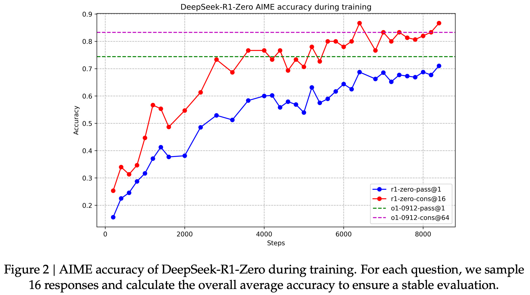
DeepSeek-R1-Zero [9] demonstrated that LLMs can learn complex reasoning behavior by applying RL training directly to a base model (i.e., with no SFT); see above. This work was the first to demonstrate that reasoning capabilities could be developed without supervised data, making the RL-Zero setup—or just running RLVR on top of a base model—a popular benchmark for RL research. Although this setup is widely used in LLM research, most RL-Zero experiments are performed using models with no data transparency, preventing proper decontamination.

“[A lack of data transparency] can lead to a myriad of issues with benchmark evaluations being contaminated; e.g. midtraining data containing the evaluation which makes spurious rewards as effective as true reward or improvements from fixing prompt templates outweighing the improvements from RL.” - from [1]

Going further, a variety of unexpected findings have been recently published by work that leverages an RL-Zero setup. For example, researchers have shown:

• RLVR with random rewards still improve model performance [12].

• RLVR with a single training example can improve performance [13].

• Base models can match the reasoning capabilities of models trained with RLVR if a sufficient number of samples are taken per prompt [14].

Understanding the cause of these findings is necessary to develop a deeper collective knowledge of RL training. Although many hypothesis exist, one possible explanation for this behavior is data contamination—these observations may simply be an artifact of evaluation data leaking into the base model’s dataset. Unfortunately, existing RL-Zero setups provide no way of validating the impact of data contamination, which makes drawing definitive conclusions from this work difficult (potentially even impossible). Olmo 3 solves this problem!

Authors in [1] release a fully open RL-Zero setup based upon Olmo 3 Base, which has fully transparent pretraining and midtraining datasets, and a new dataset for RLVR called Dolci RL-Zero. While most RL-Zero setups are single-objective (e.g., running RLVR from a base model on Math-500 is a common benchmark), Dolci RL-Zero is comprised of four domains: math, code, precise instruction following, and a mixture of all three objectives. Additionally, decontamination—or ensuring pretraining and midtraining data have no overlap with evaluation data—is prioritized, allowing more confident conclusions to be drawn from experiments with RLVR.

Notable findings. The RL-Zero setup proposed by Olmo 3 is mostly positioned as a cleaner and more reliable starting point for future research. However, authors in [1] also perform some interesting analysis using this setup. First, we see in [1] that using simpler prompt templates—mostly text-based with no special tokens as shown below—is more conducive to performant RLVR. This behavior stems from base models being primarily trained on raw text without special tokens or templates.

To achieve the best results, Olmo 3 RL-Zero performs lightweight prompt tuning with the base model to derive a simple, custom prompt with no special formatting for each RL domain. Performance of RL-Zero models is shown in [1] to improve steadily throughout RL training in terms of both training reward and held-out evaluation metrics; see below. As expected, we see an improvement in Pass@1 metrics, aligning with prior findings on RLVR15 [15]. Interestingly, we also see a slight improvement in Pass@3216 metrics, indicating that the base model learns to solve some problems that go beyond its initial reasoning capabilities.

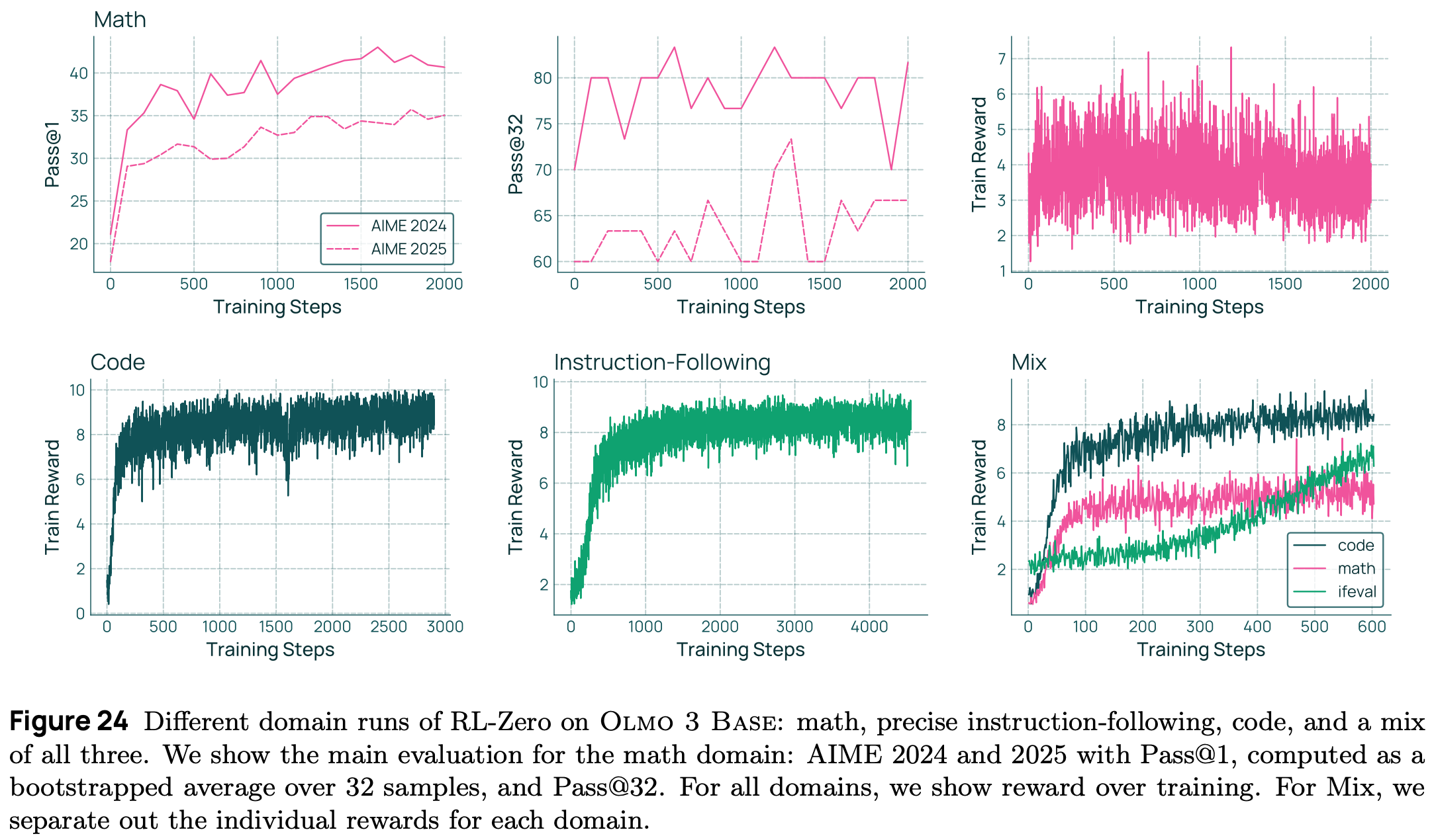
The multi-objective nature of Olmo 3 RL-Zero also presents new challenges in RLVR research. We see above that models trained over the mix of rewards from each domain improve in their performance, but they still lag behind models that are explicitly trained on a single domain. Solving this under-optimization and developing effective techniques for balancing multi-objective RLVR is a tough research problem, but Olmo 3 provides a clean and efficient—RL-Zero is cheaper than the full post-training pipeline for Olmo 3 Think!—test bed for further analysis. For example, the Dolci RL-Zero setup is used in [1] to test several changes to the underlying RL algorithm, as well as to study the impact of different data mixtures during midtraining on the downstream RL training process.

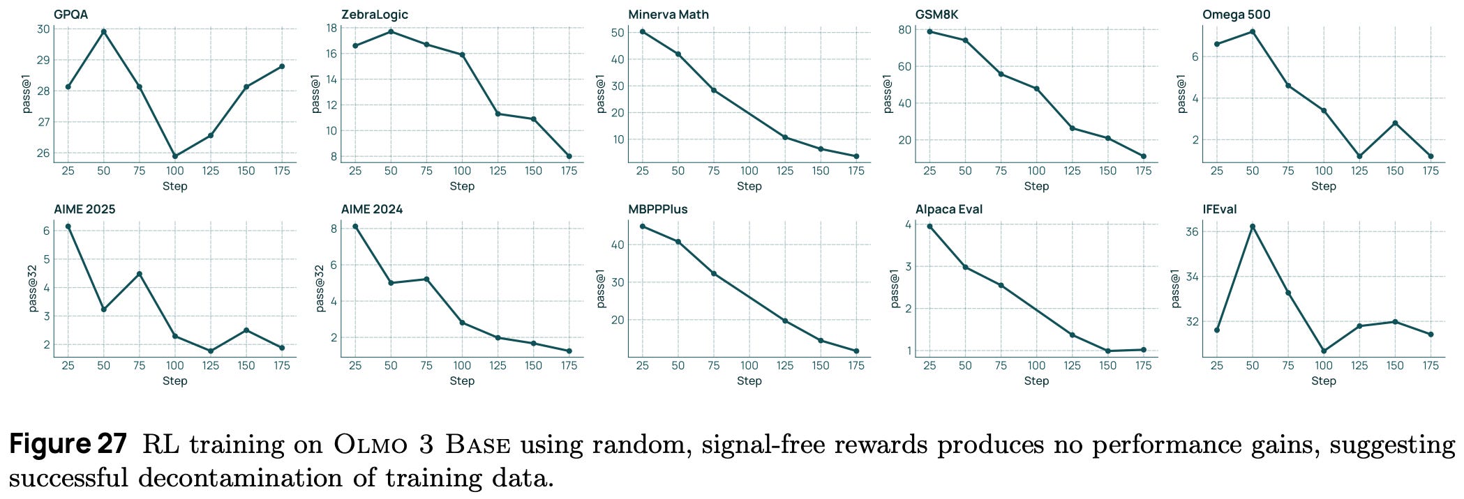
Fixing RLVR with random rewards. RLVR with random rewards no longer benefits model performance when using the decontaminated Olmo 3 RL-Zero setup; see above. Although this finding clearly demonstrates the value of fully-open models for research, the results shown for RLVR with random rewards in [12] may still not be completely a product of data contamination. As shown below, these results were only found to hold true for the Qwen-2.5 model series on the Math 500 dataset—other models and tasks did not clearly benefit from random rewards.

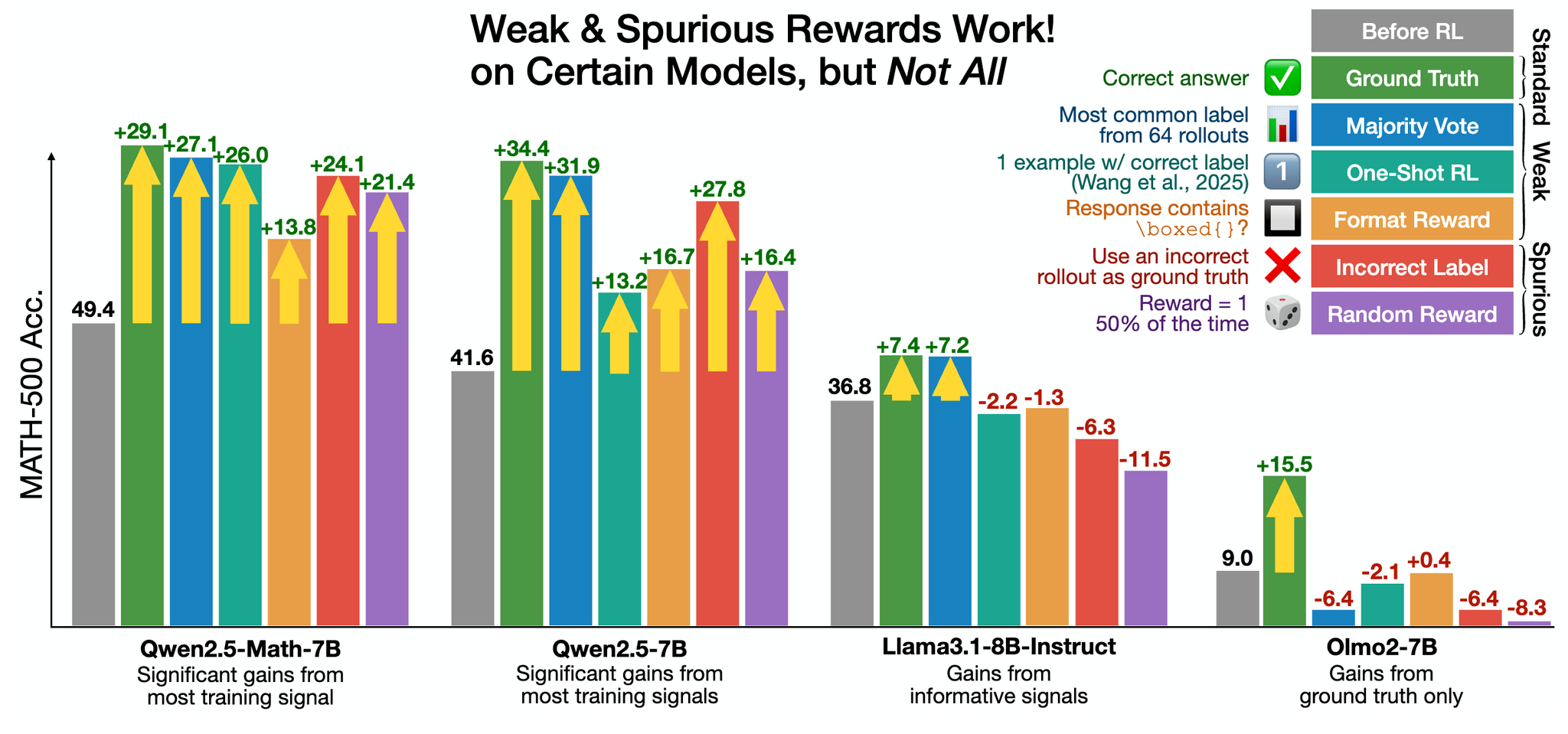
Therefore, there may be some unique aspects of Qwen-2.5—including potential data contamination—that lead to these observations, which are very hard to debug without full openness. For example, beyond data contamination, an alternative rationale exists for the performance benefit of RLVR with random rewards:

• Qwen models are very good at generating code to assist in solving math reasoning problems, and code reasoning—even when no code execution is allowed—is positively correlated with math performance.

• In the DAPO [16] paper, authors observe that entropy decreases quickly during both PPO and GRPO training. Token distributions become concentrated, so outputs are similar when you sample multiple times and existing model behaviors are reinforced (i.e., made more likely).

• This entropy collapse occurs because the clipping operation in PPO (and GRPO) restricts policy updates for low probability tokens more strictly than for high probability tokens, due to the structure of the policy ratio.

• To solve this issue, DAPO recommends a “clip higher” approach, which increases the upper bound of the clipping range in PPO so that clipping is not too restrictive of policy updates.

In the case of RLVR with random rewards, clipping can reinforce the existing behavior of performing code reasoning for solving math problems in Qwen-2.5 and, in turn, improve its performance. Although this behavior is not observed in Olmo 3, the GRPO variant used in [1] also adopts the clip higher approach from DAPO. As a result, it is unclear in this case whether RLVR from random rewards is fixed due to algorithmic changes or the lack of data contamination. However, analyzing such a property would be impossible without fully open models like Olmo 3.

Although reasoning models are very powerful, much of the real-world usage for LLMs is still based on general tasks that do not require extensive reasoning (e.g., information or advice-seeking queries). With this in mind, authors in [1] create Instruct versions of the Olmo 3 models that quickly respond to user queries without the need to output a reasoning trajectory. The training pipeline for Olmo 3 Instruct is similar to that of the Think models—it includes SFT, DPO and RLVR. Rather than focusing upon reasoning, however, the data used for Instruct post-training emphasizes multi-turn chat, conciseness of responses, and tool use.

“Everyday chat settings often do not require the inference-time scaling of Olmo 3 Think, allowing us to be more efficient at inference time on common tasks by not generating extended internal thoughts.” - from [1]

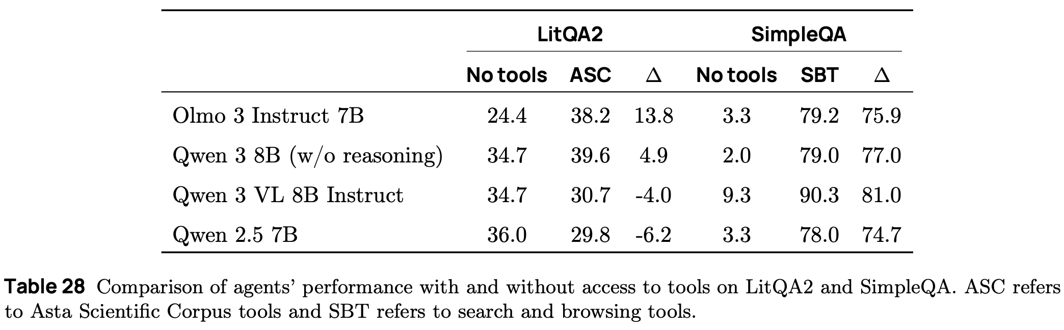
Instruct evaluation. The benchmarks used for evaluating Olmo 3 Instruct models include benchmarks from Olmo 3 Think along with a few additional benchmarks (i.e., Berkley function calling leaderboard, LitQA2, and SimpleQA) for evaluating function calling capabilities. As shown below, Olmo 3 Instruct models are found to benefit significantly from tool use, indicating that post-training has instilled correct tool usage behavior. Across other benchmarks, Olmo 3 Instruct models perform comparably to popular non-thinking models. Interestingly, Olmo 3 outperforms Qwen-3 with thinking mode turned off at the 7B scale on several benchmarks, though this gap in performance is not present at the 32B scale.

SFT. A new Dolci Instruct SFT dataset is created for Olmo 3 Instruct models that emphasizes multi-turn chat and agentic capabilities (i.e., function calling). This dataset builds upon that of Olmo 2 [3] but makes a few key changes:

• Any reasoning traces that exist in the data are removed.

• Synthetic completions are updated to use newer model generations (e.g., GPT-4.1 instead of GPT-3.5 or GPT-4).

• An extensive set of supervised function calling examples is included.

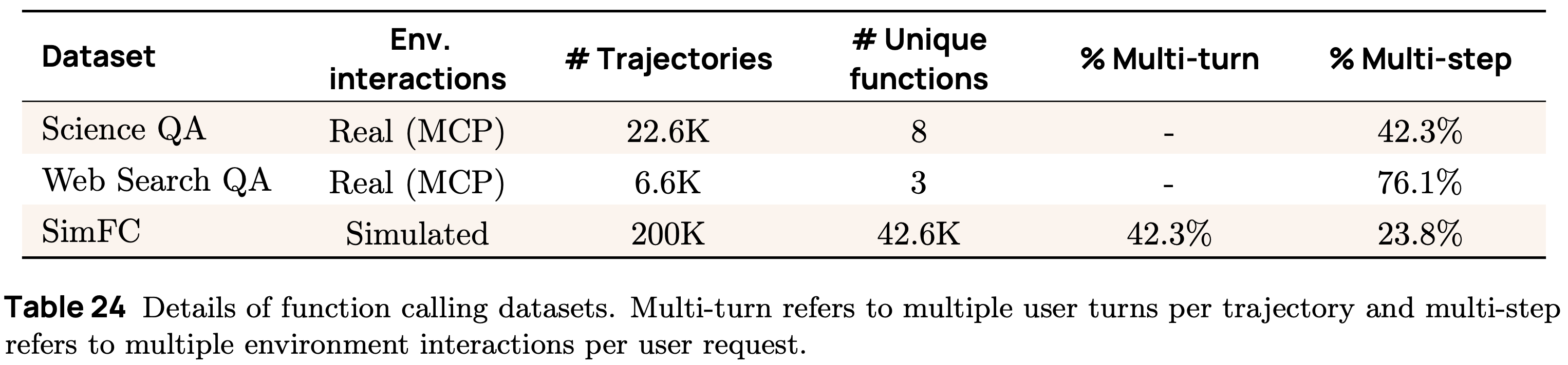
When curating function calling data, authors focus heavily upon collecting data in realistic environments, primarily MCP servers. More specifically, there are two key strategies used:

1. Real trajectories: ScienceQA and WebSearchQA datasets are created by using GPT-4.1 or GPT-5—equipped with tools for querying the internet or a corpus of scientific papers via separate MCP servers—to generate problem solving trajectories for real-world queries.

2. Simulated interactions: starting with a pool of tools and API specifications taken from public datasets, a large synthetic function calling dataset is created by prompting a pool of LLMs (GPT-4o, GPT-4.1, and GPT-5) to generate user queries, tool responses, and assistant messages.

Executable function calling environments provide valuable training data by exposing the model to complex interactions with real tool outputs—including errors. Because collecting real tool-use data is hard to scale, however, simulated environments are used to create data for a wider set of function calling scenarios; see below for details. While real trajectories are more complex, simulated data has higher tool diversity and can be used to create examples with both multiple chat turns and multiple agent-environment interaction steps.

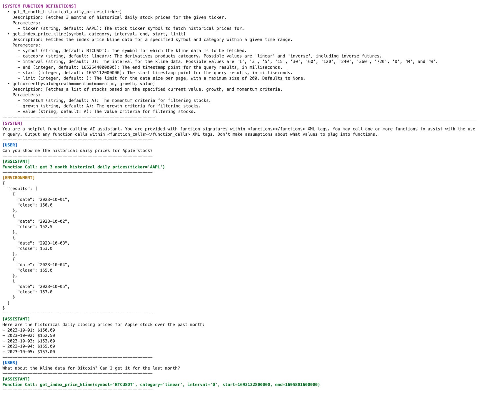
Interestingly, we see in [1] that using a unified format for function calling data is necessary for the model to perform well. Specifically, authors provide a tool spec in the system prompt, wrap tool calls in XML tags in assistant messages, and use a special environment role—represented with dedicated special tokens—for all tool outputs. An example of the unified tool format for Olmo 3 is shown below.

To obtain the final data mixture for Olmo 3 Instruct SFT, authors adopt the same strategy used for tuning the Olmo 3 Think models. Namely, we start with a base data mixture of 100K supervised examples and ablate the performance impact of each data domain that is added on top of the original dataset from Olmo 2 [3].

“We find that training our instruct model on top of the thinking SFT model both increases model performance on benchmarks… and also does not increase average model response length.” - from [1]

As we might recall from the model flow at the beginning of this overview, the Olmo 3 Instruct models are trained starting from Olmo 3 Think SFT, which the authors find to benefit performance of Instruct models.

DPO. Olmo 3 Instruct models are trained using a similar (but expanded) Delta Learning approach that is adapted from Olmo 3 Think to better prioritize general chat capabilities. Specifically, three types of preference pairs are used:

• Delta Learning is used to construct contrastive preference pairs in an identical fashion to Olmo 3 Think, but both chosen and rejected completions are generated via Qwen-3 with thinking mode turned off.

• Delta-maximized GPT-judged pairs are created by generating synthetic completions from a pool of diverse models (including at least one model that is known to be much worse than the others), scoring them with a GPT-4.1 judge, then choosing the best and worse completion as a preference pair.

• Multi-turn preferences are synthetically generated by first prompting an LLM to self-talk or synthetically generate context from an existing prompt to create multi-turn chat data, then sampling a final assistant response for this multi-turn chat via Delta Learning.

Multi-turn preferences only differ in the final assistant response, where chosen and rejected completions use models with a large quality gap (e.g., GPT-3.5 versus GPT-4.1 or Qwen-3-0.6B versus Qwen-3-32B) to generate this final turn. The GPT-judged preference data pipeline is inspired by UltraFeedback [20] but has been updated to use a more modern model pool and LLM judge; see below.

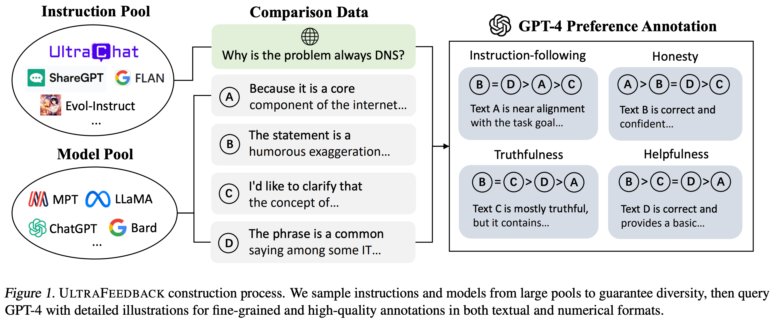
Interestingly, authors in [1] mention that naively applying the UltraFeedback approach with a modern model pool and judge performs poorly—all models in the modern pool perform well and tend to have minimal quality deltas in their output. As a solution, Olmo 3 proposes a “Delta Maximization” approach that i) ensures that at least one model in the pool is of much lower quality than others and ii) always constructs preference pairs from the best and worst completion in the pool.

“Our initial attempts to modernize the Ultrafeedback pipeline from OLMo 2 and Tülu 3 by improving the quality of the LLM judge (GPT-4o → GPT-4.1) and updating our data-generator model pool failed to yield gains and even hurt relative to the OLMo 2 preference dataset baseline.” - from [1]

Ensuring a large delta between preference pairs is found to be essential for model performance. Additionally, we see clear benefits in [1] by combining GPT-judge preference pairs with those from Delta Learning, revealing the benefit of using different preference signals. We also see in [1] that verbosity bias—or the tendency of LLM judges to prefer longer completions—noticeably impacts synthetic preference pipelines. To promote concise responses, chat-based preference pairs are filtered such that chosen and rejected completions do not differ in length by more than 100 tokens17; see below. Length control deteriorates certain benchmark scores but also improves usability, leads to better vibe tests, and is—somewhat counterintuitively—determined to be a superior starting point for RL training.

As shown in the figure above, DPO performance does not improve monotonically with more data and the optimal amount of data is task-dependent. In other words, the total size of the training dataset is a hyperparameter that must be tuned. In [1], the optimal data size and mixture is determined via a combination of:

1. Ablation experiments that combine different data sources with an 100K base mixture to determine data viability.

2. Mixing experiments that combine 50K examples from the base mixture with 50K examples from various data sources to test the impact of up-sampling a particular source of preference pairs.

3. One-off tests of hand-crafted data mixtures determined by expert intuition.

The behavior of DPO training is less predictable, and the final training strategy was determined empirically. Authors manually selected nine different mixtures to compare to a uniform sampling baseline and performed hyperparameter sweeps to determine the optimal amount of training data and learning rate. The final checkpoint is selected via a combination of vibe tests and benchmark scores.

RL. The RL training process for Olmo 3 Instruct is identical to that of Olmo 3 Think aside from a few minor modifications:

• Using less challenging datasets (i.e., by removing the most difficult tasks) in the math and coding domains.

• Removing the offline difficulty filtering step. This step is unnecessary for Instruct models due to focusing less on complex reasoning.

Olmo 3 Instruct models are trained on a mixture of general chat, math, and code data using the same RL training stack as Olmo 3 Think. However, the maximum response length is capped at 8K tokens to avoid excessively long outputs. The full RL pipeline is applied to multiple DPO models, and the final model is chosen via a combination of “final average performance, length analysis, and vibe-tests.”

AI research has traditionally been very transparent, but the level of openness has decreased during the LLM boom as top labs have focused efforts on proprietary models (e.g., GPT, Gemini, or Claude) with little transparency. Open models have always been a topic of discussion, but the level of interest in open LLM research skyrocketed with the release of DeepSeek-R1 [9]. After this release, a variety of (primarily Chinese) AI labs followed suit by releasing great models like Qwen-3, Kimi-K2, MiniMax M2, GLM-4.5, and more; see below for details.

Despite the boom in open LLM research, open LLM releases were minimal in Western countries aside from models like GPT-OSS and Mistral. Additionally, the models that were released are almost exclusively open-weights, rather than being fully open—i.e., no code or data transparency is provided. These issues inspired the creation of initiatives like the ATOM project and have driven investment into the Olmo model series. As we have seen, Olmo 3 models still lag behind their open-weight counterparts, but we should remember the following points:

1. Progress between the original Olmo model and Olmo 3 is significant.

2. No other fully-open model series has neared state-of-the-art performance.

3. The impact of Olmo 3 goes beyond just the models themselves.

The artifacts released by Olmo 3 are more than a model—they are a starting point for any aspect of open LLM research. Anyone with access to GPUs has the ability to clone and iterate upon the model flows proposed in [1]. Performing this kind of research before Olmo 3 may have required first crafting a functional training recipe, which would (conservatively) require millions of dollars in experiments.

With this in mind, resources from Olmo 3 will fuel open research for the foreseeable future. We are already seeing positive signs in this direction with models like Intellect-3, Trinity, and Mistral 3 being released immediately after Olmo 3.

Hi! I’m Cameron R. Wolfe, Deep Learning Ph.D. and Senior Research Scientist at Netflix. This is the Deep (Learning) Focus newsletter, where I help readers better understand important topics in AI research. The newsletter will always be free and open to read. If you like the newsletter, please subscribe, consider a paid subscription, share it, or follow me on X and LinkedIn!

[1] OLMo, Team, et al. “Olmo 3” https://www.datocms-assets.com/64837/1763662397-1763646865-olmo_3_technical_report-1.pdf (2025).

[2] Hugging Face Team. “Smol-LLM Training Playbook.” https://huggingface.co/spaces/HuggingFaceTB/smol-training-playbook (2025).

[3] OLMo, Team, et al. “2 OLMo 2 Furious.” arXiv preprint arXiv:2501.00656 (2024).

[4] Groeneveld, Dirk, et al. “OLMo: Accelerating the science of language models.” Proceedings of the 62nd annual meeting of the association for computational linguistics (volume 1: Long papers). 2024.

[5] Liu, Qian, et al. “Regmix: Data mixture as regression for language model pre-training.” arXiv preprint arXiv:2407.01492 (2024).

[6] Li, Yunshui, et al. “Model Merging in Pre-training of Large Language Models.” arXiv preprint arXiv:2505.12082 (2025).

[7] Pham, Chau Minh, Yapei Chang, and Mohit Iyyer. “CLIPPER: Compression enables long-context synthetic data generation.” arXiv preprint arXiv:2502.14854 (2025).

[8] Peng, Bowen, et al. “Yarn: Efficient context window extension of large language models.” arXiv preprint arXiv:2309.00071 (2023).

[9] Guo, Daya, et al. “Deepseek-r1: Incentivizing reasoning capability in llms via reinforcement learning.” arXiv preprint arXiv:2501.12948 (2025).

[10] Lambert, Nathan, et al. “Tulu 3: Pushing frontiers in open language model post-training.” arXiv preprint arXiv:2411.15124 (2024).

[11] Geng, Scott, et al. “The delta learning hypothesis: Preference tuning on weak data can yield strong gains.” arXiv preprint arXiv:2507.06187 (2025).

[12] Shao, Rulin, et al. “Spurious rewards: Rethinking training signals in rlvr.” arXiv preprint arXiv:2506.10947 (2025).

[13] Wang, Yiping, et al. “Reinforcement learning for reasoning in large language models with one training example.” arXiv preprint arXiv:2504.20571 (2025).

[14] Yue, Yang, et al. “Does reinforcement learning really incentivize reasoning capacity in llms beyond the base model?.” arXiv preprint arXiv:2504.13837 (2025).

[15] Shao, Zhihong, et al. “Deepseekmath: Pushing the limits of mathematical reasoning in open language models.” arXiv preprint arXiv:2402.03300 (2024).

[16] Yu, Qiying, et al. “Dapo: An open-source llm reinforcement learning system at scale.” arXiv preprint arXiv:2503.14476 (2025).

[17] Zeng, Aohan, et al. “Glm-4.5: Agentic, reasoning, and coding (arc) foundation models.” arXiv preprint arXiv:2508.06471 (2025).

[18] F. Yao, L. Liu, D. Zhang, C. Dong, J. Shang, and J. Gao. Your efficient rl framework secretly brings you off-policy rl training, Aug. 2025. URL https://fengyao.notion.site/off-policy-rl.

[19] Liu, Zichen, et al. “Understanding r1-zero-like training: A critical perspective.” arXiv preprint arXiv:2503.20783 (2025).

[20] Cui, Ganqu, et al. “Ultrafeedback: Boosting language models with scaled ai feedback.” arXiv preprint arXiv:2310.01377 (2023).

[21] Yang, An, et al. “Qwen3 technical report.” arXiv preprint arXiv:2505.09388 (2025).

[22] Wortsman, Mitchell, et al. “Model soups: averaging weights of multiple fine-tuned models improves accuracy without increasing inference time.” International conference on machine learning. PMLR, 2022.