Evaluating LLMs with WeightWatcher Part III: The Magic of Mistral, a Story of Dragon Kings

Recently, the Mistral models have taken the LLM world by storm. The Mistral Mixture of Experts (MOE) 8x7b model outperforms other models in it’s weight class such as LLamA 2 70B and GPT 3.5. Here’s a quick review of it’s performance on different LLM benchmarks:

And even the smaller Mistal 7b model seems to be “punching well above its weight class, taking on LLM giants”, and emerging as the Best [small) OpenSource LLM Yet. Can we understand why ?

In this post, I conjecture why Mistral 7b works so well–based on an analysis with the open-source weightwatcher tool, and drawing upon the Sornette’s theory of Dragon Kings

Here’s a Google Colab notebook with the code discussed below

A) Analyzing Mistral 7b with weightwatcher

Let’s run Mistral-7b through its paces with the weightwatcher tool. This time, however, we are going compare the standard results with one of the advanced features of the tool, the fix_fingers option (described in this earlier blog post).

Here are the steps we take:

A.1) Download Mistral-7B-v0.1 base model to a local repo:

!git clone $base_model_html

Notice that this repo contains the base model in both as both safetensors files and pytorch_model.bin files; we can remove the latter and just keep the 2 safetensors files.

A.2) Run weightwatcher with the fix_fingers=’clip_xmax’)

import weightwatcher as ww
watcher = ww.WeightWatcher()
details = watcher.analyze(model="Mistral-7B-v0.1", fix_fingers='clip_xmax')

The resulting details dataframe wlll contain 2 columns

raw_alpha: the estimated Power Law (PL) exponent alpha, without applying fix_fingers
alpha: the ‘fixed’ alpha, adjusted for fingers (i.e possible Dragon Kings)

A.3) Compare the 2 alphas

We analyze the results weightwatcher power law qualiy metric alpha by making a histogram of the raw (default) alpha, and the (fixed) alpha.

We see that the raw_alpha and the ‘fixed’ alpha look very different. The raw_alpha have a very wide distribution, with many layer raw_alpha >> 6 , with 1 even as high as 40! And the average <raw_alpha>=~5.7, which is just at the edge of the safe range (we want the average layer <alpha> in [2,.4])

The ‘fixed’ alphas, however, are very different. The distribution is much sharper, with very few ‘fixed’ alpha > 6, and the average fixed <alpha> =~ 4.8. Under the lens of the weightwatcher HTSR theory (described in our seminal paper), this is model looks much better.

A.4) Compare to other base models

Here are the same plots for the LaAMA-7b and Falcon-7b base models:

Notice that the raw_alpha and the ‘fixed’ alphas look almost identical. And the layer averaged alphas are also almost identical. So it not necessary to use the slower fixed_finger options when running weightwatcher.

So what’s going on ?

B) Fingers and Power Laws

So-called ‘fingers’ are large positive outliers that arise when computing the Empirical Spectral Density (ESD) $\rho(\lambda)$ of a layer weight matrix $\mathbf{W}$ . That is, they are usually large eigenvalues $\lambda$ of the correlation matrix $\mathbf{X}=\frac{1}{N}\mathbf{W}^{T}\mathbf{W}$ —so large that they live outside the normal and expected range of the ESD when fit to a Power Law, i.e $\rho(\lambda) \sim \lambda^{-\alpha}$ . The best way to see this is with a plot.

B.1) Plot a layer ESD with weightwatcher

Let’s pick a layer with a prominent ‘finger’ and plot the ESD.

watcher.analyze(layers=[139], plot=True)

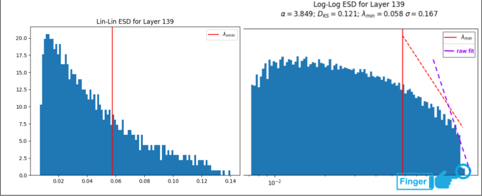
When we add plot=True, weightwatcher will generate several plots for each layer, such as the 2 plots above. The plot on the left is a histogram of eigenvalues for layer 139 (the ESD), and on a linear-linear scale, depicting a typical Heavy-Tailed (HT) ESD, The one on the right is the later ESD, this time on log-log scale, along with the PL exponent $(\alpha=3.849)$ and the quality of the PL fit $(D_{KS}=0.121)$ . The PL tail starts at the (vertical red line), and the (dashed red line) depicts the best theoretical PL fit

The finger is in the lower right side of the log-log plot, and looks like a small ‘shelf’ at the far end of the ESD. The finger consists of 1 or more spuriously large eigenvalues $\lambda_{finger}>\lambda^{max}_{fixed}$ . If we include these large $\lambda_{finger}$ in the PL fit, the result is the (dashed red line), and the alpha is unusually large, i.e $\alpha_{raw}>>\alpha_{fixed}$ . Using the fix_fingers option, weightwatcher will remove upto 10 fingers until the ‘fixed’ alpha is stable.

B.2) Stability analysis of fix_fingers option

How can we tell if the ‘fixed’ alpha is stable ? There is a plot for this too.

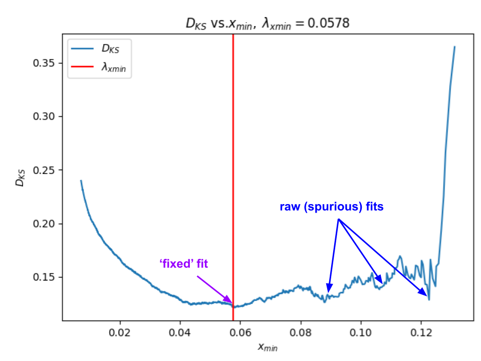
The plot on the left helps us evaluate the stability of the weightwatcher power law (PL0 fits. It plots the choice of the start of the PL tails (red line) against the qualty of the PL fit (Dks, the Kolmogorov–Smirnov distance between the data and the fit)

Good fits show a single, easily-found global minima. Bad or spurious fits have lots of close or degenerate fits

In this plot for the Layer 139 PL fit, we see a realtively convex envelope near the choice of $\lambda_{min}=x_{min}$ near the fixed fit, and lots of spurious fits that would have occured if we had included the finger in the data. (That is, there are lots of spurious fits toward the right side, indicating a smaller PL tail, i.e. the purple-dashed-line above)

B.3) Comparing alpha to other weightwatcher metrics

The alpha metric is one of a number of weightwatcher layer quality metrics. It is the most inteesting because it lets us identify the Universality class of the layer. That is , is the layer well fit $(\alpha\in[2,6])$ , overfit $(\alpha<2)$ , or underfit $(\alpha>6$ ). But alpha is also the hardest to estimate. Fortunately, we can get a rough check on our estimated alpha by comparing it to 1 or more other weightwatcher metrics.

A good metric to compare against is the rand_distance metric. This metric computes how far a layer weight matrix W is from being a random matrix–the larger the distance, the less random (or more correlated) W is. Generally speaking, smaller alpha means larger rand_distance. We can compute rand_distance using therandomize option:

details = watcher.analyze(plot=True, fix_fingers='clip_xmax', randomize=True)

alpha vs Rand_Distance

We can now plot the raw_alpha vs. rand_distance , and the (fixed) alpha vs rand_distance.

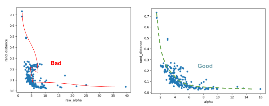
Once again, we see that the raw_alpha and the ‘fixed’ alpha cases look very different. The raw_alpha is is not even a proper function of rand_distance, and shows a stange circular trend red line. On contrast, while not a perfect relation, the ‘fixed’ alpha at least shows a noisy but proper trend green line.

Both the metrics are noisy estimators, but by cimparing them, we can see that the fixed_alpha is a more consistent estimator of the Heavy-Tailed (HT) quakity metric alpha for each layer.

C) Fingers as Dragon Kings

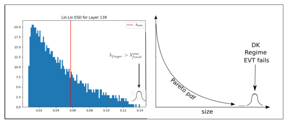
Why do we observe so many outlier eigenvalues ? Here, I posit the conjecture that these spuriously large eigenvalues correspond to Dragon Kings (DK). The Dragon King Theory was first postulated Professor Didier Sornette to explain the appearance of enormously large outliers in the power law fits of a wide range of self-organizing phenomena.

Dragon Kings (DK) are thought to arise as a result of some kind of coherent collective event or some other deterministic mechanism that can act like a dynamical attractor, accelerating the learning for the features associated with those specific eigenvectors at the far end of the ESD.

In particular, in Dragon Kings are thought to arise in quasi-critical systems exhibiting Self-Organized Criticality (SOC)–such as in the avalanche patterns observed in biological, cultured neurons!– due to the inherent dynamics and interactions within the system that push it to a critical point.

This can be due to long-range interactions and./or feedback loops, that, when activated, lead to the emergence of these extreme signatures.

When it comes to neuro-dynamics of, sometimes Dragon Kings help, and sometimes they hurt. In some cases, they are thought to suppress neural function, and, in others, they are characteristic of proper function. See this 2012 paper for a brief review; there are many recent scientific studies on this as well.

But most importantly, and in the context of training an LLM, the appearance of Dragon Kings indicates that some unique dynamical processes is generating these extreme eigenvalues and that this is fundamentally different from the goings on the normal dynamics of the SGD training processes for LLMs.

In an LLM , when do DKs hurt and when do they help ? I suspect that when they arise in the ESD like they do in Mistral-7b, they may indicate better performance. But I suspect may also appear as Correlation Traps, and, in this case, they may hurt performance.

I am postulating that it is this unique process, whatever it is, that is giving Mistral-7b (and the MOE 7x8B model) such remarkable performance. And if correct, it’s possible we could identify the underlying driving process and amplify it during training.

D) Testing the Dragon King Hypothesis with weightwatcher

WeightWatcher is a one-of-a-kind must-have tool for anyone training, deploying, or monitoring Deep Neural Networks (DNNs).

As we more and more powerful open source LLMs emerge, it will be possible to test this Dragon King Hypothesis by running the open source weightwatcher tool. I encourage you do this yourself, and / or join our Community D iscord and submit some LLMs to test.