How I Made Wine Glasses from Sunflowers—Wolfram Blog

Eons ago, plants worked out the secret of arranging equal-size seeds in an ever-expanding pattern around a central point so that regardless of the size of the arrangement, the seeds pack evenly. The sunflower is a well-known example of such a “spiral phyllotaxis” pattern:

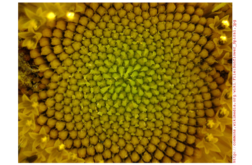
It’s really magical that this works at all, since the spatial relationship of each seed to its neighbors is unique, changing constantly as the pattern expands outwardly—unlike, say, the cells in a honeycomb, which are all equivalent. I wondered if the same magic could be applied to surfaces that are not flat, like spheres, toruses, or wine glasses. It’s an interesting question from an aesthetic point of view, but also a practical one: the answer has applications in space exploration and modern architecture.

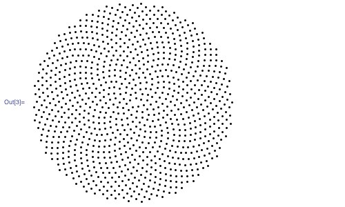
To reproduce the flat sunflower pattern mathematically, you need to know three secrets of the arrangement:

1. Seeds spiral outward from the center, each positioned at a fixed angle relative to its predecessor.
2. The fixed angle is the golden angle, γ = 2π(1 – 1/Φ), where Φ is the golden ratio.
3. The ith seed in the pattern is placed at a distance from the center proportional to the square root of i.

You can make a picture of that arrangement easily if you think in polar coordinates, with the ith seed placed at coordinate {r, θ} = {√i, i γ}:

The reason that the radial distance of the ith seed is proportional to √i is not difficult to understand. Suppose the ith seed is at distance d from the center. Then the disk of radius d contains i seeds. In order to achieve an even density of seeds, the number of seeds i in a disk must stand in constant proportion to its area πd², or:

i ∝ d²

Inverting that relationship gives:

d ∝ √i

You can apply the same reasoning to the problem of distributing seeds evenly on a hemisphere. To deal with hemispherical surfaces, it helps to think of the positions of the seeds in fixed-radius spherical coordinates {φ, θ}, where θ plays the same angular role as in polar coordinates and φ—the angular distance from the north pole along the hemisphere to a point—plays the role of r in polar coordinates. This figure shows the correspondence between polar coordinates and fixed-radius spherical coordinates:

The relationship between the area of a spherical cap and its angular radius is not the square root, as in the plane, but something else. To determine what it is, I started with the expression given in MathWorld for the area of a surface of revolution generated by rotating the parametric curve {x(t), z(t)} about the z-axis:

For a spherical cap with angular radius φ, the generating curve is the circular arc defined by

as t goes from 0 to φ.

To find the formula for the cap’s area, you don’t need to know anything about integration. You just plug the values of x, z, t₀ = 0, and t₁ = φ into the area formula, and out pops the cap’s area:

As in the planar case, I wanted i, the number of seeds, to stand in constant proportion to the area of the hemispherical cap, or:

i ∝ (1-Cos[φ])

Introducing c as the constant of proportionality, I found the relationship I sought using Solve:

The two solutions differ in the direction that the seeds spiral around the center.

The constant of proportionality c governs the density of the seeds. I solved for its value as a function of the total number of seeds n and the maximum angular radius φ_max:

Thus if I want 1,000 seeds in the entire hemisphere, which corresponds to an angular radius φ of 90°, I set c to

Putting all these results together yields the seed-covered hemisphere. The forms of the coordinate and graphics expressions here are analogous to the forms in the planar case above:

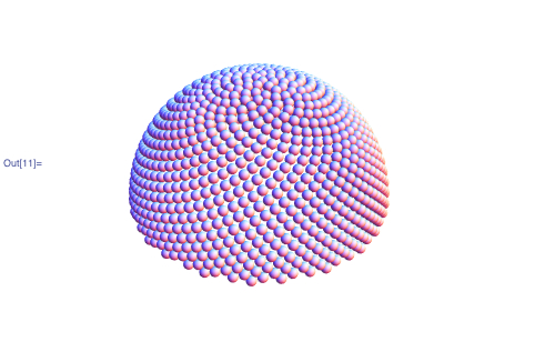
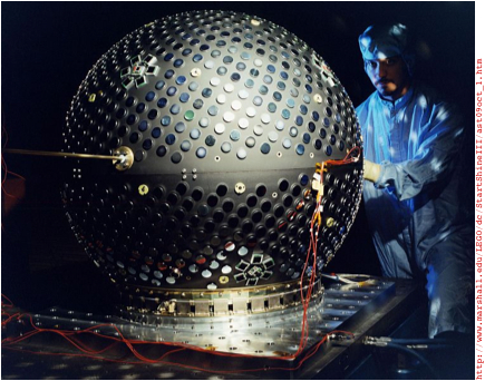
If you were building a hemispherical house, this would be the basis of a good roofing pattern, since each equal-sized shingle overlaps the joint between the two below it. Or, if you wanted to design approximately equal-area flat panels to assemble into a dome, this distribution would be a starting point. This problem of “tectonics”—how to realize curved surfaces with flat materials—is a hot topic in current architectural research. A similar problem arose in the Starshine 3 student satellite project, which required a spherical satellite to be evenly covered with reflective mirrors. The folks at the U.S. Naval Research Laboratory solved that problem with a phyllotaxic pattern.

Computing a custom function to cover each new kind of surface was an interesting mathematical journey, but a lot of work. What I really wanted was a single function that would, once and for all, distribute points evenly on any surface of revolution whose generating curve I could describe parametrically.

As with the disk and hemisphere, the secret to achieving an even distribution of points on an arbitrary surface of revolution is to make the number of points in an area proportional to the area. Unfortunately, the integral that describes that relationship often has no closed-form solution, even for simple parametric curves. But fortunately, we don’t need a closed-form solution to obtain a result. Numerical integration does nicely.

The numerical analog of the area integral above for generating functions x and z, and parameter interval t₀ to t₁, uses the NIntegrate function in place of Integrate:

This function gives area as a function of curve parameter t, but I needed the inverse relationship: given an area, I wanted to know what t is. Since I couldn’t invert this function directly, I made a table of {area, t} pairs and interpolated that to give myself a function that, from empirical evidence, approximates the inverse sufficiently well:

With those components, I assembled the function for rendering arbitrary phyllotaxic surfaces. Parameters x and z give the parametric description of the generating curve, {t0,t1} specifies the interval of the curve that generates the surface, density specifies the density of points, and radius gives the radius of the spheres that render the points.

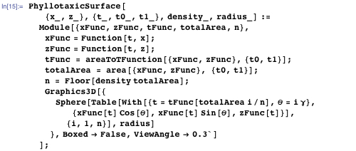
I tested the function with a covering of a complete sphere:

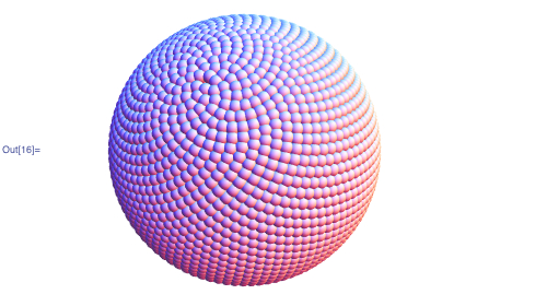
As on a sunflower’s disk, the points on the sphere group into spirals that regroup as you move from the poles toward the equator. To make that structure more apparent, I modified the rendering function so I could specify that every nth point should have a given color, and rendered spheres with n = 2, 3, …, 13. The resulting images revealed a variety of spiral structures lurking within the pattern.

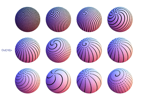
Combinations of colorings layered on top of one another show the complex interplay of spiral structures:

Since Mathematica‘s integration functions are completely general, I could explore generating curves of all sorts, including piecewise and interpolated curves. Here’s a sample of some phyllotaxic surfaces of revolution I encountered (click an image to see an enlargement):

Curious what a phyllotaxic wine glass would look like, I grabbed an image of a Peugeot wine glass from the web and used the Get Coordinates function to digitize its outline, which I fed to Interpolation to get the x and z parametric functions of the curve. This is the resulting parametric curve:

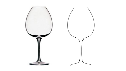
With those functions, it’s a no-brainer to make a phyllotaxic wine glass.

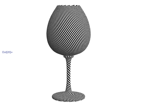
The spiral structures in this form, with its concave and convex surfaces and wide variation of diameters, were especially interesting to explore. Here’s one study that I particularly liked. It exploits the fact that when you color every seventh point, you get three distinct spirals at small diameters. I omitted the other six points entirely so that those spirals stood on their own in the stem, and gave each of them a different color. By choosing cyan, yellow, and magenta, the base and bowl of the glass are a neutral gray when viewed from a distance, and yet it shimmers almost iridescently as it moves, due to the moiré patterns induced by the patterns on the opposite sides. The magic of spiral phyllotaxis unites all the parts into one festive whole.

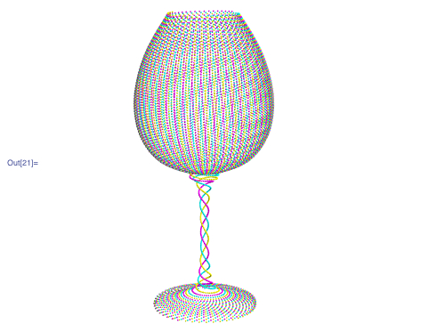
Alas, the effect requires spheres too tiny to bond together, so they’d have to be embedded in a clear glass matrix. When the day arrives that clear glass can be 3D-printed, I’ll be first in line. Meanwhile, there are plenty of other intriguing phyllotaxic surfaces waiting to be discovered.

Click here to download this post as a Mathematica Notebook.