The benefit of using Regression Adjustment (CUPED) for A/B Testing is that in certain cases it can increase the precision of the experiment’s results. However, if one isn’t intentional in the design and set up, this more powerful approach can easily lead to underpowered experiments.
What is Regression Adjustment/CUPED
One can think of regression adjustment/CUPED as a way to recycle data. If you have access to pre-experiment data that is correlated (explains some of the variability) with the upcoming test’s KPI (end-point), then by including this data when analyzing the post test data you can reduce the amount of noise, or variance in the final result. This variance reduction can be used to either increase the precision of the estimated treatment effect, or it can be used to reduce the required sample size compared to the unadjusted approach.
The amount of variance reduction is directly related to the reduction in the required sample size for given Type 1 (alpha), Type 2 (beta), and MDE. The amount of reduction relative to the unadjusted approach is based on the following relationship Var(Y_ra) = Var(Y) * (1 – Cor(Y, Covariate)2), where Y is the test’s KPI and the covariate is the pre-treatment data. For example, if the correlation of the covariate and the KPI is 0.9, then the effective variance of Y for the experiment will be 1-(0.9)2, or 19% of the unadjusted variance of Y. Since the variance of our KPI drives our sample size, this also means we need only 19% of the sample size that would be required for the unadjusted test given the same Type1, Type2, and minimum detectable effects sizes.
Wow, an 81% reduction! Huge if True! But is it true? Well, yes and no. For sure it is true relationship between the variance of Y, the covariance of Y and some covariate(s), and the sample size. However, like most things in analytics/data science, the issue isn’t really about the method but in its application and context.
For standard (Pearson-Neyman) A/B Tests calculating the required sample size requires the following inputs, the rate of Type1 control (this is the alpha, often set to 0.05), the rate of Type2 error control (this is related to the power of the test often set to 80%), the minimum detectable effect (MDE), and the baseline variance of the test metric (for binary conversion this is implied by the baseline conversion rate). So we can think of basic sample size calculation as a simple function, f(alpha, power, MDE, variance(Y)). We get to pick whatever alpha, power, and MDE we want to configure the test, but we need to estimate the variance of Y. If we underestimate the ‘true’ variance of Y, then our test will have less lower power then what we specified.
For the CUPED/Regression adjustment approach we need to add an additional estimate for the correlation between the covariate and Y. Our sample size function becomes f'(alpha, power, MDE, variance(Y), correlation(Covariate, Y)). Notice is that the effect of the correlation is quadratic. This means the any mis-estimation of the correlation when the correlation is high will have a large effect on the sample size. But this is exactly when CUPED/Reg Adjustment is most valuable.
To illustrate, if we estimate the variance to be 100 but really the baseline variance is 110. Holding our MDE and alpha fixed, underestimating the baseline variance leads to a slightly underpowered test – instead of a power of 80% our test would have a power of 76%. So less powerful, but not drastically less.
However, lets say we have some pre-test covariate data and we over estimate its correlation with Y. Let’s use as an example an estimated 0.9 correlation coefficient since this has been used by others who promote a more indiscriminate use of CUPED. However, rather than the having a 0.9 correlation, our KPI during the testing periods is closer to having a 0.85 correlation.
This results in our A/B Test having too few samples, or conversely, being underpowered since we should run the test at (-0.852), or for 27.8% of the unadjusted sample size, rather than only 19% as suggested by a correlation of 0.9. Below is the output of t-scores from simulations of 5,000 A/B tests where the actual treatment effect of the test is set exactly equal to the MDE. A test configured to have 80% power should fail to reject the null only 20% of the time. In the simulations we use the sample size suggested by a correlation coefficient of 0.9. In the simulation we ran: 1) a standard unadjusted difference in means t-test; 2) a regression adjusted t-test with a covariate that has only 0.85 correlation with Y; and 3) a regression adjusted test with a correct estimate of 0.9 correlation of the covariate and Y. Both 1 and 2 versions of the tests are under sampled for given a desired power of 80%.
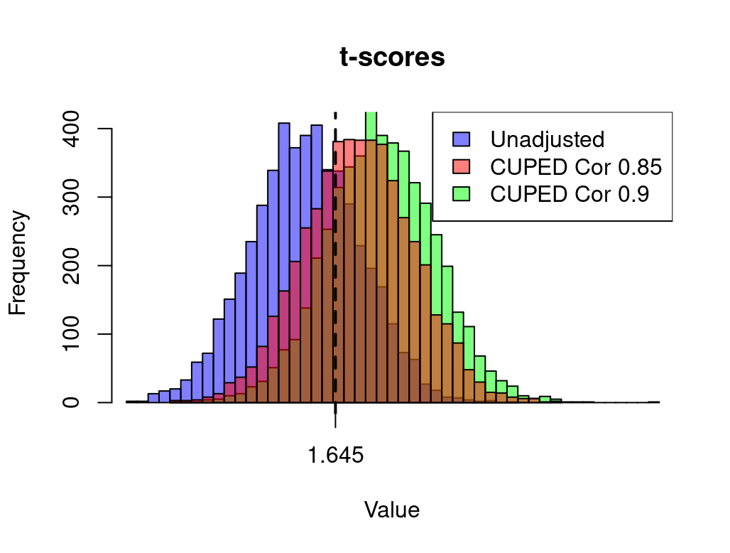
The unadjusted A/B tests (Purple) are shifted to the left of the 1.645 critical value with 70% of all tests failing to reject the null for the one tailed 95% confidence test. This make sense because we only have 19% of the required sample size. The regression adjusted test with the correct estimate of 0.9 (Green) has just 19.8% of the tests to the left of the 1.645 critical value, which is the expected 20% fail to reject rate (80% power). The regression adjusted tests using a covariate that has only 0.85 correlation rather than 0.9 (Red) is shifted to the left such that we fail to reject 34% of the tests, for a power 66%. So even though we have data that can massively increase the precision of our results versus the unadjusted t-test, we still wind up running under powered tests. Which of course is highly ironic. It means that exactly when CUPED/Regression adjustment are most useful, if we are not careful in our thinking and application, it is also exactly when we are mostly likely to increase our chances of running highly underpowered tests.
Why? Our estimates of correlation are based on sampling the data we have. Often A/B tests have different eligibility rules, so each test, or family of tests, will need to have its own correlation estimate. Each estimate requires a faithful recreation of these eligibility rules to filter on the existing historical data. As we generate many of these estimates, each on subsets of historical data, it becomes more likely that we have a nontrivial share of them with under estimates of correlation. This increases the odds of mis-estimation even if the underlying data is stationary. If the data is not stationary, then it is even more likely we will run underpowered tests.
Of course this doesn’t mean don’t ever use regression adjustment/CUPED. For example, here a simple, admittedly ad-hoc fix might be to just use a slightly more conservative estimate when the correlation estimate is very high especially when its based on limited historical data for finer sub-sets of the population. However, it does suggest that the promises about more advanced methodologies are often broken in the details, and that one should be intentional and thoughtful when designing and analyzing experiments. Good analysts and good experimentation programs don’t just follow the flavor of the day. Instead they are mindful of trade-offs, both statistical as well with the human factors that can affect the outcomes.