At Conductrics, two of our guiding principles for experimentation are:
Principle 1: Be mindful about what the problem is, preferring the simplest approach to solving it.
Principle 2: Remember that how data is collected is often much more important than how that data is analyzed.
Often, in the pursuit of ‘velocity’ and ‘scale’, the market will often over promote ever more complex solutions that tend to be both brittle and increase compute costs. Happily, if we are thoughtful about the problems we are solving, we can find simple solutions to increase velocity and growth. The Power Pick Bandit introduced by Conductrics in this 2018 blog post is a case in point.
In this follow up post we will cover two significant extensions to the Power Pick Bandit:
1) Extend the power pick approach for cases when there are more than two arms;
2) Introduce a two step approach that controls for Type 1 error when there is a control.
Power Pick Bandit Review
As a quick review, the power pick bandit is a simple, near zero data analysis, multi-armed bandit approach. The bandit is set up just like an A/B Test, but with one little trick. The trick is to set alpha, the type 1 error rate, to 0.5 rather than something like 0.05. This will reduce the number of samples by almost a factor of four. Even though there is almost nothing to it, this simple approach will find a winning solution, IF THERE IS ONE, at a rate equal to the selected power. So if the power is set to 0.95 then the bandit will pick the winning arm 95% of the time.
Power Pick Multi-Arm Case
Let’s say that rather than selecting between two arms we had 10 arms to select from. How can we best apply the power pick approach? The naive case is to just multiply the per arm sample from the 2 arm case by 10. Let’s say we have a problem where the expected conversion rate is 20%. We want our bandit to have a 95% probability to select an arm if it is 5% better than that average. In the case below Arm 2 has a true conversion rate of 21% and all the other arms have a true rate of 20%.
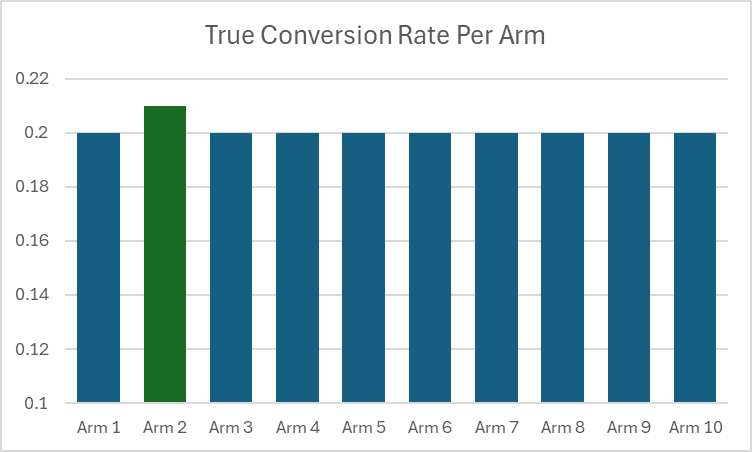
We decide to use the power pick approach and we naively use a power of 0.95. Using our sample size calculator we see we will need approximately 8,820 samples per arm. Running our simulations 10k times, with 88,200 samples per simulation we get the following result:

The arm with the 21% conversion rate is selected 77% of the time, and one of the 9 other arms are selected 23% of time. Not bad but not at the 95% rate we wanted.
Adjusted Power
In order to configure the many armed bandit to select a winner at the desired probability we borrow the Bonferroni adjustment, normally used for FWER in A/B tests with multiple comparisons, and apply it to the power. To adjust for the desired power we divide the Beta (1-power) by 1 – minus the number of arms in the problem. For our case we want the power to be 0.95, so our adjusted power is
Adj Power = 1-[(1-0.95)/(1-10)]=0.9944.
Using the Adj Power forces us to raise our sample size to 210K from 88K. After running our simulations on the larger sample size we select the best arm 96% of the time (Bonferroni is a conservative adjustment so we expect slightly better error control).

While the number of samples needed is much greater than in the naive approach, they are still fewer than if we had used a naive A/B test approach.

The adjusted power approach uses 40% less samples than a simple 10 arm A/B Test. Beyond being a useful tool to easily optimize a choice problem when there is no type 1 error costs, it highlights that most of the efficiency of using a bandit vs an A/B Test is not in any advanced algorithms. It is almost entirely because the A/B Test has to spend resources controlling for Type 1 errors.
But what if we do care about Type 1 errors?
The Two Stage Adjusted Power Pick
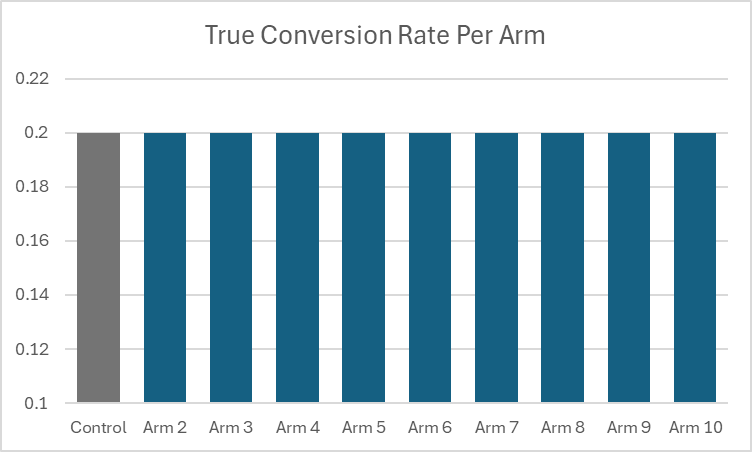
Let’s adjust our problem slightly. Instead of trying to select from 10 arms, where we don’t care about type 1 error, let’s imagine that one of the arms is an existing control. We have a set of 9 other arms and we just want to quickly discover if any one of them might be a promising result.
Since we have an existing control, we want to ensure that we control for false positives at the 5% rate.
The standard way to do this is to run a single Bonferroni (or pick your favorite adjustment for FWER) A/B test. To estimate the sample size we adjust the alpha of 0.05 to 0.05/(10-1)=0.0056. To keep the simulation time down, we use a power of 0.8. The number of samples for the Bonferroni corrected 10 arm A/B test is 372k.
However, the Bonferroni approach uses extra samples to test each alternative against the control. But growth teams often have situations where there is a large set of potential alternatives where they want a way to first quickly bubble up the best option and then test that option against the control. For these cases we propose the Two Stage Power Pick approach. First, run an adjusted power bandit on all 10 arms, including the control. If the control is the winner, stop and move on to some other problem. If the winner is not the control, then run a two arm A/B Test between the control and the winner.
There is one additional technical consideration. In our case we want the joint power over both stages to equal 80%. If we ran stage one at a power of 95% and the stage two power at 80%, the joint power would be only be 76% (0.95*0.80=0.76). To account for this we adjust the second stage power so that the product of stage one and stage two power equals the desired power. This can be achieved by dividing our desired joint power by the stage one power. So if we want a joint power of 0.80 and the stage one power is 0.95, the adjusted power for stage two is 0.80/0.95 = 0.8421.
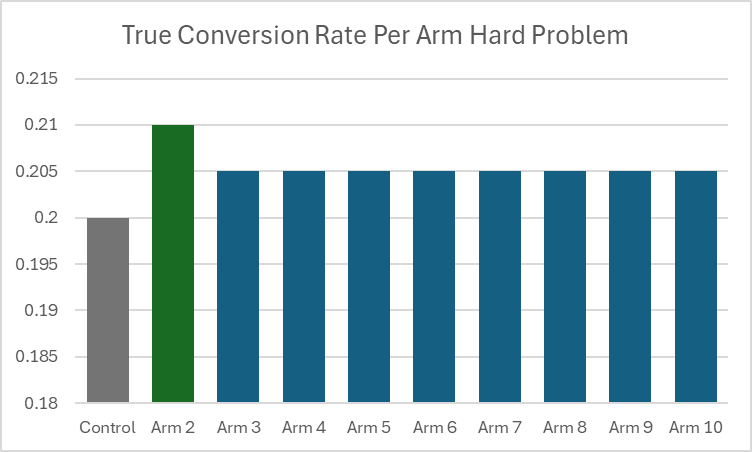
The following results are when there is a single arm that has a 21% conversion rate when all the other arms, including the control have a 20% conversion rate. Notice that both approaches have a power of at least 80% as expected. However, for this case, on average, the two step approach needs only 256K, which is 30% less data than the Bonferroni A/B test .

What about when none of the arms are different from control?
After running 10k simulations we see that both approaches control type 1 error at or below the 5% level. Also note that the average sample size for the 2 Step approach is slightly less under the null than when there is a ‘best’ arm. This is because on average 10% (more generally 1/k where k number of arms) of the time the control will ‘win’ the first step and the procedure will terminate.

Of course there is no free lunch. There are trade offs around how the various approaches will perform depending on the relative payoffs between the various arms. In cases where it is the control that has the highest conversion rate of all the arms, then the two step approach will terminate early more frequently, resulting in a sample size that approaches the samples needed just for the first stage (because the control will get selected as the winner of the first stage with high probability) . However, the two step approach is less robust in cases when there are sub optimal arms that are both better than the control but are less than the specified minimum detectable effect. For example a case where one arm is better than the control by the MDE, but all of the other arms are better than the control by one half of the MDE.
Comparison of Results
In the chart below, we have three scenarios: 1) Where there is just one arm that is MDE better than the control with 8 other ‘null’ arms; 2) our hard case from the above chart, with all the alternative arms better than the control, but with just one arm a full MDE better; 3) An easier case where there are two arms MDE better than the control, with 7 other ‘null’ arms.
In the first scenario both approaches achieve the desired power of 80%. For the hard problem in the second scenario both the two stage adjusted power approach and the Bonferroni adjusted A/B Test have reduced power. The two stage approach is however less robust, with an achieved power of 52.4% vs a power of 69.5% for the Bonferroni. In the third case where there are two arms better than the control by the MDE and all the other arms equal to the control both methods achieve at least 80% power, but the Bonferroni approach is better able to take advantage of this easier problem. Of course this additional sensitivity of the adjusted power approach is balanced by requiring much less data – 30% less when it runs both stages and over 40% less when it terminates early when the control is the best arm.

For many situations, especially for growth teams, where there is a large set of possible solutions and the team would like to increase their testing velocity, using the adjusted power approach can be a very useful tool. For basic bandit problems it provides a simple, low tech, easy to manage approach that is surprisingly effective. For discovery type tests, where we want to quickly surface a promising challenger from a large set of options before testing it against an existing control, the two step adjusted power test can be a faster alternative than the standard multiple comparisons adjusted A/B Test.
If you have any questions or are interested more in what we are working on over here at Conductrics please feel free to reach out.