Can advanced AI lead to negative economic growth?

This essay is about the role of economic demand in AI-driven growth forecasts. The premise is simple: if advanced AI (or AGI, which I will use interchangeably) automates most labor and the wage share collapses, who will buy the increased output? If firms anticipate weak demand, will they keep investing and producing? Will the economy face a gap between potential and realized output, and actually shrink?

Let’s take a simple parable, suggested to me by Tom Cunningham, that illustrates this logic. Imagine there’s an island with 100 workers and 10 capital owners. Everyone consumes two types of goods, fish and coconuts. Workers catch fish and harvest coconuts using nets and ladders provided by the capital owners. Workers are paid wages for their labor and spend everything they earn on the two goods. Revenue goes directly to the owners. The owners are wealthy, and because a person can only eat so many fish and coconuts, they consume 10 of each per day and have their fill.

Now let’s say fishing gets automated. Someone invents self-operating nets that catch fish without workers. Workers are fully displaced from fishing and move on to harvesting coconuts, which still requires labor. Workers still earn wages, and because fish has now become much cheaper, they may be even better off than before as their earnings can now buy them more of the two goods. Output rises in this economy: owners respond to demand by investing in nets and labor is now fully devoted to coconuts.

But suppose someone invents an automatic harvester that picks coconuts, and there are enough of these harvesters to fully replace workers in the groves as well. Both sectors are now fully automated and the workers cannot be re-deployed elsewhere. They earn nothing and spend nothing. What happens to output? Well owners are still satiated with 10 fish and coconuts each. That’s 200 units of total demand. Machines are sitting sitting idle: they could produce 10,000 units, and even more if owners would invest it building more. But why would the owners bother if there’s no one to buy the output? In this economy, full automation led to negative growth because of demand collapse.

This sort of logic has been articulated many times before. I first encountered it in Jaron Lanier’s “Who Owns the Future”, where he argues that increasing automation may disenfranchise the majority of the population; the economy shrinks because most people cannot buy what technology can produce. Martin Ford makes a similar argument in his books “The Lights in the Tunnel” and FT Book of the Year “Rise of the Robots: How Artificial Intelligence Will Transform Everything”. For example, in the former Ford writes “once full automation penetrates the job market to a substantial degree, an economy driven by mass-market production must ultimately go into decline. The reason for this is simply that, when we consider the market as a whole, the people who rely on jobs for their income are the same individuals who buy the products produced.”

Tom Cunningham has been running a prediction aggregator of AI-driven growth. Although there is substantial disagreement in the forecasts, with economists towards the lower end and technologists towards the higher end (e.g., Elon Musk predicting double-digit growth within 12-18 months), all of the forecasts are positive. Reading the economics papers that the forecasts are based on, as well as other theoretical work on the topic, I did not see the possibility of AGI-driven demand collapse discussed. And while there has been a lively debate about the implications of automation on inequality, the potential for negative growth has not come up.

So given the popular intuition described earlier, I thought it would be useful to work out whether conditions for negative growth exist, and if they do, whether they end up being ones we should be worried about.

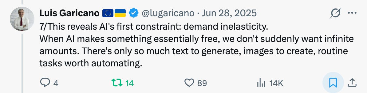
It turns out that these conditions do exist, and more importantly, they’re not too crazy (at least on their own). I’ll discuss two possibilities here. The first is based on the combination of satiated preferences and the redistribution of wealth from workers—who spend most/all of their income on consumption—to the wealthy and relatively satiated capital owners. The idea that satiated preferences can impact AGI-driven growth is motivated by an excellent post from Luis Garicano: as in the initial example, it is possible that at some point people will feel like they have enough of a product and become a lot less motivated to buy it regardless of how cheap it becomes. If broad automation shifts income from un-satiated high-spending (high MPC) workers to the satiated low-spending (low MPC) capital owners, this can trigger a Keynesian demand collapse that contracts the economy.

The intuition is very similar to the notion of indebted demand from Mian, Straub, and Sufi, where heterogeneous MPCs mean that redistribution from borrowers towards savers can reduce aggregate demand in the economy; this is because borrowers tend to have higher MPCs than savers. The case of AGI-driven automation is more extreme: If the majority of people do not have the money to buy what is being produced, while those who do are already satiated, then firms will cut back on production and capital investment, and economic output will decrease. Automation expands the technological frontier of what could be produced but ends up shrinking realized output.

While the set of conditions for “demand collapse” are largely on preferences, Benzell and colleagues’ “Robots Are Us” shows that you can also get negative growth (which they term immiserating growth) through capital decumulation. In their model, automation can lead to lower savings due to collapsing wages, and this lower savings translates to shrinking capital stock. The entire process takes place in an overlapping generations framework, so that while automation makes the current generation who has savings and capital better off, future generations are left worse off.

So what did I learn from these exercises, will advanced AI actually lead to negative economic growth? Probably not. Writing down these models and working through them shows that the conditions needed for growth to actually turn negative are likely too unrealistic to hold in practice. To me, this illustrates why economic theory is so important: without writing down the model, it would be difficult to push back on the strong intuition motivating the parable I started with. But as the formalism makes clear, the specific assumptions required for negative growth—as opposed to merely disappointing growth—are likely too extreme.

At the same time, I think it is worth considering the impact of labor displacement on demand. With less extreme assumptions, automation can depress demand and push AI-driven growth toward the lower end of current forecasts. The good news is that there are policy tools to counteract these forces are readily available, as I discuss in the last section of the essay. For example, a system like a sovereign wealth fund where people get a stake in the growing share of capital will ensure that demand remains robust without disincentives for investment and innovation (unlike, say, a tax on AI companies). Such funds already exist, both in the US (the Alaska Permanent Fund) and elsewhere (e.g., the United Arab Emirates manages a huge sovereign wealth fund).

I also want to emphasize that changes in economic output and growth are separate from considerations of welfare. For example, the welfare consequences of AGI-driven redistribution can be very negative even if the economy continues to grow; alternatively, even if growth turns negative, welfare may be positive if the gains are not entered into the growth accounting. See, for example, the work by Erik Brynjolfsson and Avi Collis for example.

Finally, a few caveats. First, I am not a macroeconomist. While I am a consumer of research in the field, I have not worked heavily with these sorts of models since graduate school. My hope with this essay is to start a conversation about the role of demand in AI-driven growth projections, and I plan on treating this post as a “living document” to be updated. Second, there is currently a lively debate happening on whether AGI will actually lead labor share to collapse (see, for example, here and here) This essay does not ask whether AGI will lead to the collapse of labor share. Rather, it examines the consequences of such displacement, asking the question of how much does labor have to shrink to generate negative growth.

Okay, with that out of the way, let’s dive in.

I’m going to first consider a setting where labor becomes largely obsolete so that the people left with income are mostly capital owners. Before diving into the model, it’s worth understanding why many supply-side economics papers predict a boom from AGI. The key component is Hulten’s Theorem, which says that the aggregate benefit from improving any input equals that input’s share of total costs. If a sector’s labor accounts for about 10% of GDP, then driving labor costs to zero will lead to a 10% increase in GDP. So if advanced AI reduces the costs of labor tremendously, we should expect economic growth to jump quite a bit.

But in the settings where Hulten’s Theorem is typically applied the economy smoothly adjusts to produce the technically feasible output. This works fine when we’re talking about modest productivity improvements in specific sectors. For example, when phone operators were automated away in the first half of the 20th century, the economy kept on humming along (although the phone operators themselves did not fare so well. This is because displaced workers were able to move to new sectors. When agriculture became more efficient, many farmers moved to factories. When factories became more automated or moved overseas, people moved to services. There was always somewhere for human labor to go.

But if AGI reaches its theoretical ideal then it will automate multiple sectors in a very short amount of time; displaced labor will have few places to be re-deployed. This can potentially generate a collapse in demand that keeps the economy from achieving its technological capacity.

Here is a simple model (details of the model can be found here). There are two types of agents: workers and owners with their proportions of the population being theta and (1-theta), respectively.

Workers earn wages; owners earn returns on capital and scarce resources like land and energy. The main behavioral assumption is that these groups have different marginal propensities to consume (MPCs):

That is, workers spend most of their income on consumption while owners do not. Historical estimates suggests that this is indeed the case: Wealthier owners of capital have lower MPCs because many of their consumption needs are already satisfied.

Firms produce differentiated goods using a CES production function combining labor and a non-labor input (capital, land, energy):

where:

Consider what happens when advanced AI leads to a collapse in labor intensity alpha. That is, when AGI arrives, alpha falls from alpha_0 to some much smaller alpha_1. What happens to the economy?

Before deriving the main result, it’s worth being explicit about what kind of model this is. The production function (equation 2) describes what the economy could produce, i.e., the technological frontier. In this short-run framework (dynamics are considered later on), actual output is determined by demand, not by full use of available factors. Firms observe demand and hire or obtain the labor and capital needed to meet it, leaving excess capacity and machines idle if demand is lacking.

This type of Keynesian demand-determined equilibrium is pretty different from the classical supply-determined one. The production function tells us about costs and factor shares, but the level of output is pinned down by aggregate spending. When later on you see Y = C, this means that firms produce only what consumers want to buy.

A natural question is if some households have marginal propensities to consume less than one, where does their unspent money go? In the static model here, savings do not factor back into economic growth accounting. This is a strong assumption made to illustrate the intuition. In a frictionless world, excess savings would lower interest rates until investment absorbed the surplus. The section labeled “The Stagnation Trap” extends the model to include investment and shows that the demand collapse result survives if there is a floor on how low interest rates can go, the familiar secular stagnation or liquidity trap scenario. For now, the static model isolates the pure redistribution channel by assuming investment is fixed at zero.

The first thing to note is that prices don’t fall to zero. Even if labor is free, firms still need energy, land, raw materials, and computing infrastructure. These inputs have positive prices because of physical scarcity. So while unit costs fall, they remain strictly positive.

The second key element is the satiated preferences. When prices fall, consumers can afford more stuff, but they don’t necessarily buy everything they can afford. There’s a limit—at some point, people have enough toasters, food, and cars. You can model this through the use of a “satiation” term:

that approaches a finite ceiling as prices fall:

You can think of this as the maximum consumption any household would want even if goods were essentially free, similar to a bliss point but without the falling utility on the other side.

To see the intuition, consider the history of artificial lighting, which Garicano uses to motivate his post. In 1800, lighting a home cost a day’s wage. By the 1990s, the real price had fallen by a factor of 40,000. Did we consume 40,000 times more light? Of course not; our demand for light is finite. At some point, every room is bright enough, and extra lumens have near-zero value. The lighting sector’s technological triumph made it economically tiny as a share of GDP.

With all of this in place, we can state aggregate consumption as:

where s_L is labor’s share of income and kappa_0(P) is the price-dependent baseline consumption (bounded by satiation). The term AMPC(s_L) is the aggregate marginal propensity to consume, which is a weighted average of workers’ and owners’ MPCs.

In the goods market equilibrium, Y = C, which implies:

You can probably see where this is going. AGI does two things:

• It lowers prices P, which raises kappa_0(P’) relative to kappa_0(P), but only up to a certain amount given satiation.

• It substantially decreases labor share s_L, which lowers AMPC (since workers’ high MPC is replaced by owners’ low MPC), shrinking the Keynesian multiplier 1/(1-AMPC). Note this is the same logic as in the idea of indebted demand, where redistribution from high MPC borrowers to low MPC savers decreases aggregate demand.

Real GDP falls after AGI if:

Putting it in words: GDP falls when the multiplier shrinks by more than baseline consumption can expand. The increases in aggregate demand (numerator) can’t keep up with the redistribution effect (denominator).

In the technical note, I include a derivation (h/t Usama Polani) that can be used to tell us how much AI needs to displace labor in order to generate negative economic growth. Let the consumption expansion factor be defined as:

When AGI lowers prices, g > 1 captures the boost to baseline consumption. From (6) we can derive a labor share threshold s_L^{*}(g), where a demand-driven output fall occurs whenever s_L’ < s_L^{*}(g).

The threshold s_L^{*}(g) has a natural interpretation: for any given consumption expansion factor g, it is the minimum post-AGI labor income share required to prevent demand-determined output from falling, given the assumed MPC heterogeneity.

Several properties follow immediately:

• When g = 1 (no price-induced consumption boost), the threshold equals the pre-AGI labor share: s_L^{*}(1) = s_L. Any decline in labor share reduces output.

• As g increases, the threshold s_L^{*}(g) falls. Larger price-induced gains in baseline consumption can offset larger redistributions away from workers.

• For sufficiently large g, the threshold can become negative, meaning economic output rises regardless of how far labor share falls.

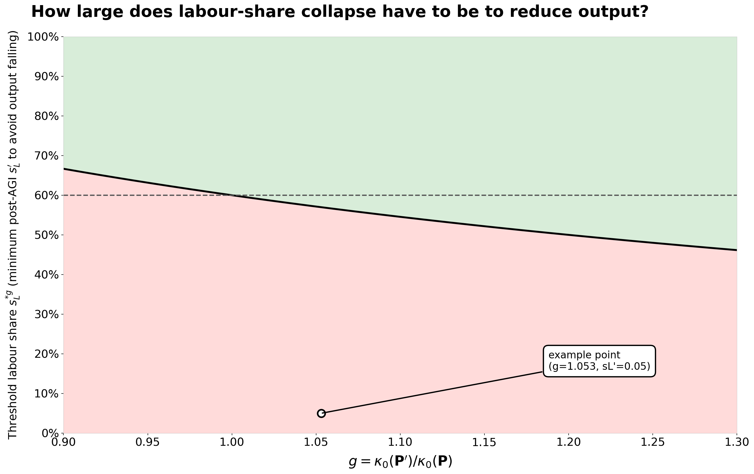
In the figure below shows the relationship between the consumption expansion factor and labor share. The green region represents points where the economy continues to grow after AGI; the red region corresponds to where it shrinks. The more that consumption increases in response to lower prices, the more of labor that needs to be automated in order to induce negative growth.

Let’s go through a numerical example. Suppose pre-AGI:

• Labor share: s_L = 0.60

• Workers’ MPC: kappa_1_Z = 0.90

• Owners’ MPC: kappa_1_O = 0.20

• Baseline consumption: kappa_0 = 38

• Real GDP: Y = 100

Post-AGI, labor share collapses to s_L’ = 0.05 and prices fall dramatically by 30% (so P’ = 0.7). Due to satiation, baseline consumption rises only modestly to kappa_0(P’) ~ 40$. Meanwhile, the aggregate MPC falls from:

to:

Post-AGI GDP becomes:

This point is highlighted in the figure above. Real GDP falls decreases by nearly 48%, despite dramatic productivity improvements. The economy can technically produce much more—potential output is quite high—but it won’t because there isn’t enough demand for it.

Now let’s add some dynamics. The static model assumes that savings do not turn into investment, which is a pretty big simplification. In reality, when owners spend less, their savings can lead to more investment. This may help balance out the drop in demand. If capital owners choose to save instead of spend, they may invest those savings, so total output does not have to decline.

Let’s think about a dynamic model that includes capital accumulation. In this case, Y = C + I, and how much firms invest depends on what they expect future demand to be and how much it costs to borrow money. The new equilibrium condition is:

Can investment take in the extra savings from owners with low MPCs and stop the demand from collapsing? This depends on whether interest rates can drop enough to encourage sufficient investment.

Define the “natural rate” of interest as the rate that balances the goods market when the potential output of the economy is realized. When AGI sharply reduces the labor share, the amount people want to save goes up a lot, since more income goes to owners who save more. To keep the market balanced, investment must increase to use up these savings, which means interest rates need to fall. But if interest rates cannot go any lower—because of things like the zero lower bound, a lack of safe assets, or other obstacles—the natural rate might not be possible to reach.

If the needed natural rate is lower than what is actually possible, the economy cannot reach the technological frontier just by changing interest rates. Instead, output drops until the amount people want to save at the new, lower income matches the amount that can be invested. This is sometimes called the multiplier-accelerator spiral: weak demand leads to less investment, which reduces the capital stock, and that makes demand even weaker. The economy settles into a low-output steady state, even though it could produce much more.

A simple example shows how big the effect can be. Using the same MPC values as before and a capital-output ratio of 3, the economy before AGI keeps Y = 100 with investment making up 15% of output. After AGI causes the wage share to collapse, keeping Y = 100 would need investment to be over 50% of output, which is not realistic unless there are many more profitable investment options. Instead, output drops to about 37, and the capital stock shrinks by a similar amount.

The main point is that a collapse in demand does not need savings to vanish. It happens when savings are greater than what the economy can use for investment at any possible interest rate. Regular monetary policy does not help here. Lowering interest rates does not work because the issue is not the cost of borrowing. The real problem is that workers do not have income to spend, and owners already have more than enough. This is exactly what happens when most income goes to households who already have all they want to consume and see little benefit from investing more.

There are a few reasons to doubt that AGI will lead to negative growth. The numerical example and the accompanying figure illustrate this. Depending on the baseline consumption response to lower prices, labor share needs to collapse by a lot in order to actually decrease economic output. But even aggressive AGI timelines assume a gradual transition, with humans retaining comparative advantage in tasks requiring physical presence, interpersonal trust, or regulatory requirements for human judgment. See work by Joshua Gans and Avi Goldfarb for example. A more realistic scenario might see labor’s share fall by a smaller margin and in certain sectors (e.g., trucking, which I will discuss in a future post). This could be a serious drag on growth but not reverse it.

Second, the idea that people will be fully satiated at some level of consumption is a big assumption. While it’s true that there’s a limit to how much artificial light people want, history shows that people keep finding new things to want. Air conditioning, international travel, cosmetic surgery, and video games are all examples of new types of consumption that past generations never imagined. AGI could create new categories too, like personalized AI companions, virtual reality experiences, or life extension services, which could attract spending from wealthy owners.

Third, and relatedly, funds that are saved through AGI do not get reinvested into capital because of firms’ anticipated lack of consumers. But this again precludes the creation of new markets and products that those who have the funds will want to buy.

Fourth, the model assumes that institutions never change. In real life, political pressure will likely lead to changes like more social insurance, shorter work weeks, or a sovereign wealth fund, before GDP growth turned red. The idea that institutions would completely fail is, hopefully, not realistic.

My view is that this model captures a real force that will moderate AGI growth expectations, but the specific conditions for negative growth represent an extreme case that policy and behavioral adjustment would prevent. Note that this says nothing about welfare: eliminating the main source of income of a large share of the population, especially when that share is lower down on their utility-of-consumption curve to begin with, can potentially have a large negative welfare consequence. But the strong conditions of the model required to generate negative growth suggest that we should not look for the welfare consequences of AGI in the GDP numbers.

Seth Benzell and colleagues’ “Robots are Us” model describes a slower, more gradual way that AGI can shrink the economy. Instead of a sudden drop in demand, the model shows how automation can slowly weaken the economy’s ability to build up physical capital. Over time, this leaves everyone worse off, even though technology keeps improving. (Side note: Benzell explains that the model was partly inspired by Asimov’s “The Caves of Steel,” where robots do almost all the work, wages stay low, and growth stalls because the government does not reinvest in expanding automation.)

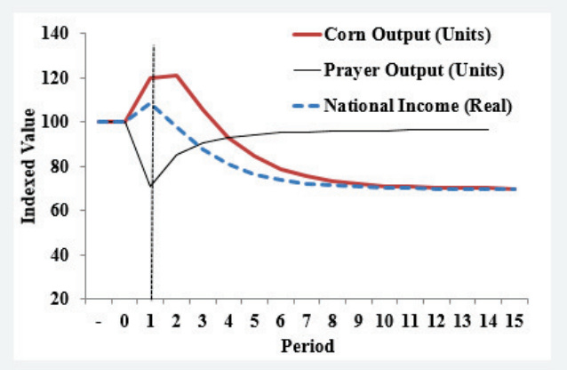
The basic framework uses a standard overlapping generations (OLG) model. There are two goods: Corn, which is an automatable product made with capital and code, and Prayers, a non-automatable service that needs human labor. Corn represents mass-produced goods, while prayers stand for interpersonal services such as therapy, coaching, spiritual guidance, or artisanal crafts that, for now, cannot be automated.

There are two types of workers: high-tech workers who write code and low-tech workers who only produce prayers. Each person lives for two periods, working when young and consuming when old. This OLG setup matters because people save for retirement, and those savings fund the economy’s capital stock.

Here is how code builds up over time:

When delta increases, it means technology is improving so software lasts longer, thanks to things like better documentation, more modular design, or moving from paper tape to silicon chips.

The key mechanism is that old code ends up competing with new coders. After Junior, the chess program, easily beats every human at chess, there’s no reason to hire anyone to improve chess code. The problem is solved, and Junior’s code makes chess programmers unnecessary.

When delta goes up and code lasts longer, there is an initial boom. Coders are in demand because their work sticks around. Wages in tech rise, people save more, capital builds up, and the economy grows. But as more legacy code piles up, the value of new code drops. Why pay for new coders when you can use the huge library of existing software? In the end, most coding jobs are just about maintaining and updating the current code base.

As coding becomes less profitable, high-tech workers switch back to the prayers sector. Now, both groups earn less because wages in both areas are connected by workers moving between them. This is where the OLG structure matters: when workers make less, they save less. Since their savings fund the economy’s capital, less saving leads to less investment and a smaller capital stock.

The model can end up in a bleak situation where:

• Technology (code stock) is higher than ever

• Physical capital is lower than ever

• Output is lower than the pre-automation steady state

• Everyone is worse off

Benzell and colleagues call this outcome “immiserating growth,” which means technological progress that actually makes everyone worse off.

The broadest way to understand the mechanism for immiserating growth is that if AI lowers the national saving rate enough, technological progress can actually reduce output. In formal terms, immiseration happens when:

The first term shows the direct productivity gain from AI, while the second term reflects the indirect effect through capital accumulation. Immiseration happens if the negative effect on capital outweighs the direct productivity gain.

The OLG structure offers a clear way for this to happen: AI shifts income from patient young savers to impatient older consumers. However, similar outcomes could also result from other factors, e.g., AI rat-race competition that stops long-term resource building, or higher catastrophe risks that make everyone value the future less.

In the Cobb-Douglas case, the steady state depends on two main equations. Whether immiseration occurs depends on whether the capital-to-code ratio k = K/A drops enough when delta increases:

When k drops, the marginal product of capital goes up because capital is scarcer than code, but wages go down since labor is more plentiful. If wages fall too much, saving drops, capital shrinks even more, and the economy declines further.

The paper’s simulations show this is possible. With a saving propensity phi = 0.2 and delta rising from 0 to 0.7, real national income initially rises 7.8% then falls to 4.2% below its starting point. The capital stock falls by 65%, wages fall by 25%, and long-run welfare drops by 16.5%.

The conditions for immiserating growth show that it is hardly guaranteed. The same simulation with a higher saving rate (phi = 0.85) produces permanently higher welfare. The key is whether saving is high enough to maintain the capital stock despite falling wages. This shows why the OLG structure is important. In a model where agents live forever, capital shortages fix themselves because higher interest rates encourage more saving. In OLG, though, young people save based on their wages instead of what the economy needs. If wages fall, savings drop too, which makes the capital shortage worse.

Benzell et al point out that there is no irrationality or Pareto failure here. Technology really does make the first generation better off. The issue is that you cannot improve their situation further without hurting future generations. The process only needs redistribution from patient to impatient agents, and OLG is just one way this can happen. The “prayers” sector is not necessary either. Even in a fully automated economy, the saving-rate effect still works as long as income moves from savers to consumers.

However, there are reasons why long-term negative growth is unlikely. Each “period” in the model lasts 30 to 40 years, which gives plenty of time for policies and behaviors to adjust. Similar to the critique of the demand collapse model, the non-automated sector can grow to take in workers who lost other jobs, rather than staying the same. Pension funds, sovereign wealth funds, and proactive governments could also react to expected capital shortages in ways the model does not consider.

Like the demand collapse model, I see the immiserating growth framework as pointing out a real economic force that can potentially lower growth expectations. However, the exact scenario leading to decreased output depends on several assumptions that are likely to be violated in practice.

What should we take from these models?

To me, the channels outlined here temper my expectations that AGI will lead to explosive growth. Both models point out mechanisms—like demand collapse due to redistribution, or loss of capital from savings differences across generations—that supply-side models overlook.

However, the conditions needed for negative GDP growth seem too extreme. Both models assume almost total automation of human work, no policy response, and that institutions do not change. While each of these assumptions might make sense on its own, it is hard to believe all four would happen at once.

Ultimately, the extent to which advanced AI leads to economic growth depends on the technology itself, but also on the rules and systems that shape how its benefits are distributed within the economy. Addressing demand-side issues is not only important for workers; companies should also be concerned about these issues. If demand falls, there will be fewer customers, and even the most efficient AI-driven business cannot succeed if people cannot afford to buy its products.

To me, the most promising approach is to make capital ownership more widely shared. If more of the country’s income goes to capital instead of labor, it is important to spread capital ownership across the population. A sovereign wealth fund that pays dividends to a country’s citizens would provide income and keep demand steady, without taxing profits or innovation in ways that could slow growth. This idea is not extreme; it is similar to privatized Social Security plans where workers get shares of capital instead of relying on future workers’ wages. Alaska’s Permanent Fund is a real-world example, as is the case of the UAE.

It is important that these ownership stakes cannot be sold or traded. If people could sell them, some would likely cash out their shares because of bad choices, urgent needs, or scams, and end up with no labor or capital income. Making the stakes inalienable gives everyone a lasting share in the economy’s output. While this approach is somewhat paternalistic, in a future where most people no longer earn wages, letting people lose their ownership could have serious consequences.

Interestingly, the two models discussed here point to different policy priorities. The demand collapse model suggests giving income to workers who are likely to spend it, while the immiserating growth model suggests giving income to people who save and invest. Broad capital ownership could help with both: it gives families money to spend, which keeps demand up, and also gives them assets to invest, which supports growth.

The good news is that these solutions are not unusual. Sovereign wealth funds, citizen dividends, and broader ownership structures are familiar policy tools. Importantly, they do not share the disincentive properties of taxes that could themselves blunt growth and investment.

Thanks are due to numerous people who provided feedback on multiple drafts, many useful conversations, and comments on thoughts I sent their way. These include Brian Albrecht, Seth Benzell, Tom Cunningham, Steve Hou, Séb Krier, Usama Polani, Daniel Rock, Anthony Lee Zhang, and especially Luis Garicano.