Newton's method and fractals

Martin Pergler, 99.11.25. Handout for Calculus 151/30, fall 99.

    Newton's method is a method for iteratively approximating the roots of a function f(x) using the derivative. In other words, you want to find a value x such that f(x)=0, and you do it by guessing and then refining your guess over and over again.
    If the function is quite simple, you may be able to do some algebra to find a root x exactly. For instance, if f(x) is a quadratic polynomial, you can use the quadratic formula. If f(x) is a degree 3 or 4 polynomial, there are messier formulas which work as well. But if f(x) is a higher degree polynomial or a more complicated function, there is no analog to the quadratic formula, i.e. there is no systematic process to algebraically determine the roots exactly. You have to approximate, and Newton's method is one way of doing this.
    We'll start with considering Newton's method over the real numbers, i.e. when x is always real and so is f(x). However, we'll see that the situation becomes much more interesting when we let x and f(x) be complex numbers. For simplicity, we'll use f(x)=x³-1 in this write-up. Of course, we all know that x=1 is the only real root, and there are two other complex roots x = -1/2 + (3^1/2/2) i = -0.5 + 0.866 i and x = -1/2 - (3^1/2/2) i = -0.5 - 0.866 i.        (1) [Exercise: verify this], and so we don't really need Newton's method in this example. However, even in this simple case we already get pictures which are quite complicated enough!

The Newton's method formula

The idea behind Newton's method is simple. Let f(x) be a differentiable function. Take a starting "guess" for a root and call it x₀. Draw the tangent line to f(x) at x₀, and figure out where this tangent line crosses the x-axis. This is the next guess x₁ for a root. If f(x) were equal to its tangent line, x₁ would actually be a root of f(x), of course. In general, this is not the case. However, the tangent line approximates f(x) for x near x₀, and so we hope that x₁ is not "too far off" from a root of f(x), in particular hopefully closer than x0. Repeat the process with x₁ instead of x₀ to get the next approximation x₂, and so on. Thus each x_n is determined by f(x_n-1) and the slope of the tangent line at x_n, which is f '(x_n-1). The appropriate formula [Exercise: do this or look up in the textbook] is x_n= x_n-1- f(x_n-1) / f '(x_n-1) (2)

Examples for f(x)=x³-1 over the real numbers

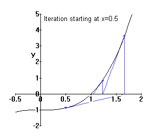In this case, formula (2) becomes x_n = x_n-1 - (x_n-1³-1) / 3x_n-1². (3) Let's start with the guess x₀=0.5. Iterating formula (3) gives the sequence shown at right. We are getting closer and closer to the root x=1, so things are working well. In fact, you can see from the picture that any guess x₀>1 will quickly converge to the root x=1. In fact, if you randomly pick almost any x₀, chances are x_n will converge to x=1. Notice, however, that if x₀ is close to 0, then the tangent line there is almost flat and x₁ will be blasted way out to the right on the x axis. This is not much of a problem, though, since x₂ will be pushed rapidly back, as the graph shows for x₁=1.7 (approx.).

If we choose x₀=0, we are in trouble, since the tangent is horizontal, f '(x₀)=0 and formula (*) crashes. Furthermore, if we choose a different x₀ which eventually "lands" on x_n=0, we have the same problem. The graph at right shows this in red for x₀=-1.434, which crashes in 2 steps in this manner. There is an infinite sequence of "bad" negative points like this. Note that if we choose an initial guess very close to such a bad point, x_n will eventually become close-but-not-equal-to 0, and then x_n+1 will get blasted way out to the right and from there eventually converge to x=1. The closer we began to a bad point, the more steps it will take to get "reasonably close" to x=1. [The previous statements all require some work to prove. Skipped.] An example of this is shown in blue.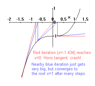

Using complex numbers

What happens if we now allow x (and f(x)) to be complex numbers rather than just real numbers? Can we get the other complex roots? Though it is beyond the scope of a first-year calculus course, it is possible to define the derivative over complex numbers just as for real numbers, so formula (2) makes sense. It turns out that polynomials are all complex-differentiable, and the complex-derivative is (surprise!) the same as the real-derivative. So formula (3) still holds, even though the geometry is much more complicated. (In part since x is now in some sense 2-dimensional and likewise f(x), so we need to think in 4 dimensions!)
We change notation and call the variable z instead of x, and write x and y for its real and imaginary parts, so that z = x + i y. Starting with some (complex) guess z₀, we can apply the formula and get a sequence z_n, which hopefully converges to a (complex) root. Here is what happens for three values of z₀ close to 0.5 + 0.5 i.

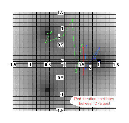
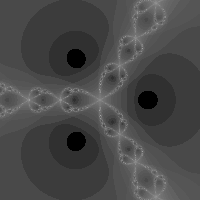
The picture shows that one choice (blue) converges to the real root, but another (green) converges to one of the other complex roots. But if we choose precisely z₀ = 0.539 + 0.417 i (determined with some effort!), then z₁= 0 .539 - 0.417 i, and z₂=z₀! So we get into an infinite cycle back and forth between these two values and do not converge to any root. This is a different sort of "bad point" than the ones we found on the negative real axis, when f '(x)=0.
Incidentally, the grey shading in the graph represents |f(z)|. The dark squares are near the roots, when |f(z)| is 0, and the squares are progressively lighter as |f(z)| gets bigger, and hence f(z) gets "further from 0".

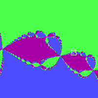
The basin of attraction picture

A natural question to ask is as follows: as z₀ varies, which root does z_n converge to and when does it not converge? This is shown by coloring in the diagrams below: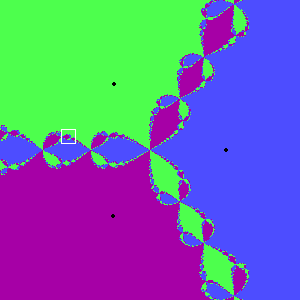

    The first is for x and y ranging from -2 to +2, and the remaining two are successive magnifications of the part of the image in the white square. The three roots have been arbitrarily assigned the colours blue, green, and purple.
    Where are the "bad" points? We already saw there are points of no convergence, shown by red trajectories in previous sections. These are isolated points however, and not easy to hit without trying, and so don't show up in a "random" calculation. It can be proven (check this. ref?) that precisely at any "corner" between blue, green, and purple, there is actually an isolated red (bad) point. In fact, it so happens that on the straight line between any two points of different colours lie points of any other colour! (and hence infinitely many points of all colours).
    The above pictures are called Newton basin of attraction images for f(z)=z³-1.

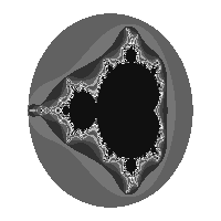
Fractals

Fractals are images which generally exhibit the following related 2 properties: [details beyond the scope of the course]

They exhibit small-scale self-similarity, i.e. little sections appear to be "almost" copies of a larger section of the image, one which contains the little section in question.
They are in some sense "infinitely complicated" on a small scale.

The discussion in the previous section shows that Newton basins of attraction are fractals. You may have seen another mathematical fractals such as the Mandelbrot set (at right), which also arises from an iterative system somewhat similar to equation (2). Fractals of various sorts occur in many ways in nature, for instance in modelling the earth's surface or in living objects such as trees and ferns. In recent years, they have also been used to create super-realistic computer graphics in movies!

Some other related pictures...

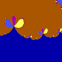
Here is the Newton basin of attraction picture for f(z)=z⁵+6z+1, which cannot be algebraically factored. However, f(z) is "almost" the same as g(z)=z(z⁴+6), which would have roots z=0 and 4 symmetrical roots around the origin for the quartic factor. Hence we are not surprised the roots and the basin of attraction picture is "almost" symmetrical.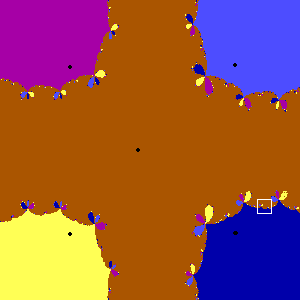

Finally, instead of colouring our picture by which root z₀ converges to, we can instead measure how many iterations of formula (2) it takes to get z_n "really close" to the root it converges to ("really close" means to some fixed small distance). Then we get pictures like the one at right (for our cubic example). The closer the colour is to white, the more iterations are required. It clearly shows how complicated the situation is near to the rays dividing the plane into 3 sections.

Playing around more...

You can interactively draw Newton basin of attraction pictures for any polynomial you want (by specifying its complex roots) by visiting David E. Joyce's Newton Basins site at Clark University.
You can also draw all sorts of fractals on a DOS/Windows computer using Fractint. They also have lots of fascinating pictures at another page on the same site.
If f(x) has several real roots, you can still draw interesting pictures using only real numbers by coloring the points on the x (real) axis according to which root they iterate to. There is a Java applet that does this at this site