Gauss's Principle of Least Constraint

$ \newcommand{\1}{\mathbbm{1}} \DeclareMathOperator*{\argmin}{argmin} \DeclareMathOperator*{\argmax}{argmax} \newcommand{\x}{\times} \newcommand{\Z}{\mathbb{Z}} \newcommand{\Q}{\mathbb{Q}} \newcommand{\R}{\mathbb{R}} \newcommand{\N}{\mathbb{N}} \newcommand{\E}{\mathop{\mathbb{E}}} \renewcommand{\bar}{\overline} \renewcommand{\epsilon}{\varepsilon} \newcommand{\nullset}{\emptyset} \newcommand{\set}[1]{\{#1\}} \newcommand{\TODO}[1][TODO]{\textcolor{red}{#1}} \renewcommand\qedsymbol{$\blacksquare$} \newcommand{\consaccel}{\text{ConsistentAccel}} \renewcommand{\t}{\widetilde} \newcommand{\grad}{\nabla} \newcommand{\Fconst}{F_{\text{const}}} $

This note is about a formalization of classical mechanics due to Gauss. Gauss noticed that, roughly, the constrained motion of masses is as close as possible to their unconstrained motions, while still satisfying the constraints. For example, a pendulum bob would naturally fall straight down, but is constrained to a circle by its string -- so its true acceleration will be as close as possible to straight down, while still remaining on the string. This generalizes to essentially any constrained system. Specifically, to find the true accelerations of masses in a constrained system, we first find the accelerations as if they were unconstrained, and then “project” to the closest acceleration that satisfies the constraints. \[a_{\text{true}} = \argmin_{a \in \text{ConsistentAccelerations}} ||a - a_{\text{unconstrained}} ||^2_M\]

This formulation (which also holds in generalized coordinates) is another nice extremal principle in physics, and is the basis of some recent fast rigid-body physics simulations (MuJoCo), using convex optimization.

In this note, we state, prove, and discuss Gauss's principle, assuming minimal prior knowledge. We use it for a double-pendulum simulation just for fun.

Introduction & Motivation

The problem we are concerned with is constrained dynamics . That is, we have some masses interacting with external forces, and subject to constraints on their state (eg, a ball constrained to move on a track, or two masses connected by a rigid bar). We want to know how they move.

Of course, this is the general problem of classical mechanics, but we are focusing on how to deal with constraints. Directly applying Newtonian mechanics can get very messy when dealing with kinematic constraints, since it requires solving for all the intermediary constraint forces. Often, we are not interested in what forces are required to enforce the constraints, we just want to know the eventual movement of the masses. (For example, a ball rolling along a curved track – we are not interested in the forces required to keep the ball on the track, just in the eventual motion of the ball). Re-formulations of mechanics (such as Lagrangian mechanics, and Gauss's principle) give us “implicit ”ways of dealing with constraints.

Organization. We first setup the problem and notation, then in Section we state Gauss's Principle and give several examples. In Section we formally define the notion of "consistent accelerations" required for Gauss's Principle. Finally, we give a proof of Gauss's Principle in Section . We conclude with remarks, historical references, and open problems.

Setup and Definitions

We specify the configuration of our system by some collection of coordinates $\vec X \in \R^n$. For example, for $k$ masses we could specify the positions of all the masses $\{x_i : x_i \in \R^3\}$. We can also use generalized coordinates instead of spatial ones, for example the angle of a pendulum.

A constrained system (to us) is one where the configuration $X$ is constrained to lie on a manifold. For example, we may have the constraint $x_1 = -x_2$, or if two masses are connected by a rod of length $\ell$, the constraint $||\vec x_1 - \vec x_2||_2 = \ell$. Here, we will consider only constraints that do no net work on the system (this is the case for most natural physical constraints).

Given a configuration $X$ on the manifold, let $T_X$ be the set of possible velocities of the system at configuration $X$, which are consistent with the constraints. Notice that $T_X$ is a subspace, and is in fact exactly the tangent space of the manifold at $X$. (We will see examples soon). Our condition that constraint forces do no net work is exactly the condition that (in inertial coordinates) the collection of constraint forces $\Fconst$ is orthogonal to $T_X$.

The state of a system is given by the positions and velocities $(X, \dot{X})$.

The mass matrix is the matrix $M$ such that $\frac{1}{2}||\dot{q}||^2_M = \frac{1}{2}\dot{q}^TM\dot{q}$ is the kinetic energy of the system, where $\dot{q}$ is the generalized velocities. (Such a matrix always exists when the mapping $q_i(r_1, \dots r_n)$ between generalized coordinates $q$ and spatial coordinates $r$ is time-independent).

Our goal is: Given the constraint manifold and the current state $(X, \dot{X})$ of a system, find the accelerations $\ddot{X}$. This determines the entire trajectory $X(t)$.

This goal is the analog of Newton's law ($F=ma$) – it specifies the local evolution of a system.

Gauss's Principle

Gauss's principle is:

The set $\consaccel$ is defined and discussed further below.

For example, if we describe our system in inertial, spatial coordinates, and there is an external (non-constraint) force $\vec F_i$ acting on mass $m_i$, then the true accelerations satisfy:

\[\{\vec a_1, \dots, \vec a_n\} = \argmin_{\{\vec a_1, \dots, \vec a_n\} \in \consaccel} \sum_i m_i ||\vec a_i - \frac{\vec F_i}{m_i}||^2\]

Examples

Pendulum

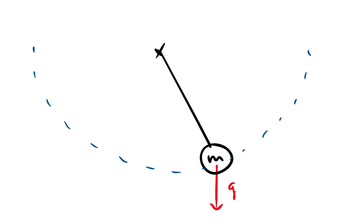
Model the configuration space as the position of the mass $(x, y) \in \R^2$, constrained to lie on the manifold $C = \{(x, y): x^2 + y^2 = 1\} \subset \R^2$. The mass matrix is simply $M = \begin{bmatrix} m &0\\ 0 &m \end{bmatrix}$. The unconstrained acceleration of the mass is simply $g$, straight down by gravity.

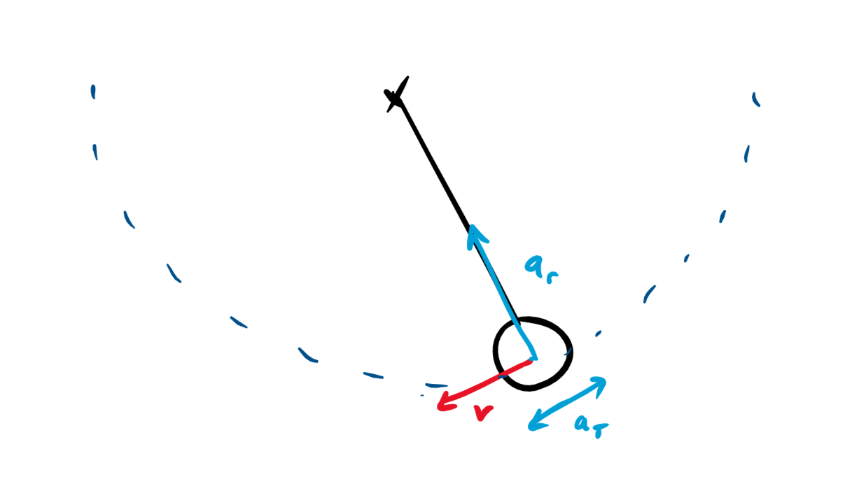At a given state (position and velocity $v$) of the mass, let us consider the space of consistent accelerations. The fixed velocity determines the radial/centripital acceleration ($a_r$, in blue), so the only freedom is in the tangential accelerations ($a_T$). Thus, the consistent accelerations are exactly those with the given radial acceleration, and arbitrary tangential acceleration. (This will be discussed further below.) The projection of $g$ onto the consistent accelerations (as dictated by Gauss's Principle) is equivalent to considering the tangential component of gravity.

Note that we could not have directly used the angle of a pendulum as a generalized coordinate when applying Gauss's Principle, since we can't express the unconstrained acceleration of the pendulum in terms of only this coordinate. Thus, Gauss's Principle requires us to work in an ambient space that includes even "off-shell" trajectories of the constrained system. However, it is still possible to use generalized coordinates in our representation, as we will see below.

Double Pendulum

In practice, it is still possible to use generalized coordinates in our computations, though we will need to map it back to spatial coordinates. This is useful for simulations, because we can use coordinates that implicitly respect constraints. For example, for the double pendulum, we can represent the configuration space by the two angles $\vec \theta = (\theta_1, \theta_2)$. The set of consistent accelerations in $\theta$-space is simply all of $\R^2$, since the angular accelerations can be arbitrary. Thus, we just need to translate this set back into spatial coordinates. The spatial coordinates $\vec r = (\vec r_1, \vec r_2)$ of the masses are functions of $\theta$: $\vec r_i(\theta_1, \theta_2)$. Now, at a given state $S = (\theta_1, \theta_2, \dot{\theta_1}, \dot{\theta_2})$, we have $$ \ddot{\vec r} = Q_S \ddot{\vec\theta} + \vec b_S $$ for some matrix $Q_S$ and vector $b_S$ depending on the state. This follows simply by differentiating $\vec r(\vec \theta)$. Thus, we can express the set of all kinematically feasible accelerations as the affine space $$\consaccel_S = \{Q_S \ddot{\vec\theta} + \vec b_S : \ddot{\vec \theta} \in \R^2\}$$ This is extremely convenient, because we can now apply Gauss's Principle to directly find $\ddot{\vec\theta}$, the generalized accelerations: $$A = \argmin_{A \in \consaccel_S} ||A - A_\text{unconstrained}||^2 \iff \ddot{\vec\theta}_{true} = \argmin_{\ddot{\vec\theta} \in \R^2} ||Q\ddot{\vec\theta} + b - A_\text{unconstrained}||^2 $$ This is, presumably, something like what MuJoCo does.

Just for fun, here is an example implementation of the above (plus some dampening for stability). Try some random configurations. On the left is a phase-space plot of $\theta$ vs $\dot{\theta}$ ($\theta_1$ in blue, $\theta_2$ in red).

Sliding Blocks

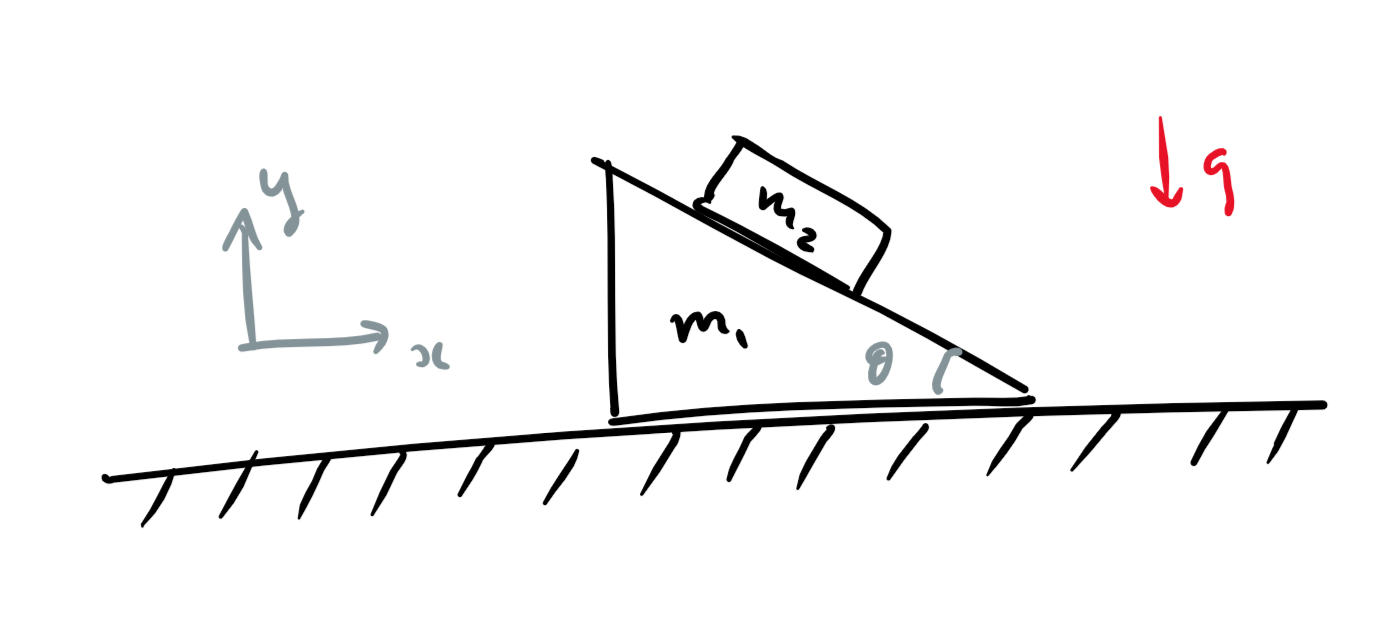Take the ambient space as the $x$ coordinate of mass $m_1$, and the $x, y$ coordinates of mass $m_2$: $(x_1, x_2, y_2) \in \R^3$. The 2-dimentional constraint manifold (for appropriate choice of orgin) is defined by $\{(x_1, x_2, y_2): \tan \theta = y_2/(x_1-x_2)\}$, expressing the constraint that the block remain on the wedge. The mass matrix is again diagonal, since we are using inertial coordinates: $M = diag(m_1, m_2, m_2)$.

And More...

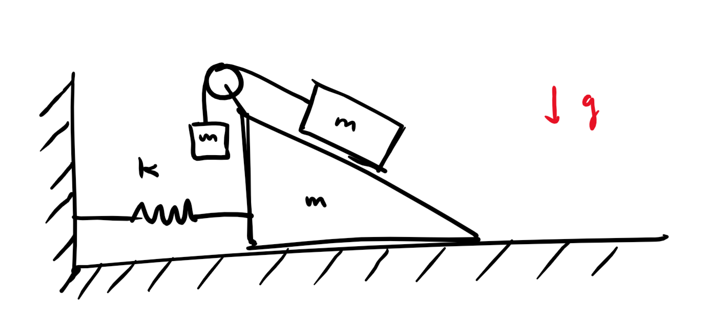(Left as an exercise for the reader). Note that we can handle internal non-constraint forces, such as springs -- this is just incorporated into the unconstrained accelerations.

Consistent Accelerations

Here we define the set $\consaccel$, and show a property that will be required in the proof of Gauss's Principle.

We define $\consaccel$ in order to move from constraints on the positions of masses to constraints on their accelerations. This can be done by differentiating the manifold constraint at the current state.

Formally, given the current state $(X, \dot{X})$ of a constrained system, define the “consistent accelerations ”as the following set. Consider all trajectories $\t X(t)$ which are kinematically feasible (lie on the constraint manifold), and agree with the current state at $t = 0$: $(\t X(0) = X, \dot{\t X}(0) = \dot{X})$. The consistent accelerations are the set of all accelerations for these feasible trajectories: \[\consaccel_{X, \dot X} := \{\ddot{\t X}(0)\}\]

The following property is important:

For example, consider the consistent accelerations of a pendulum at its bottommost point: 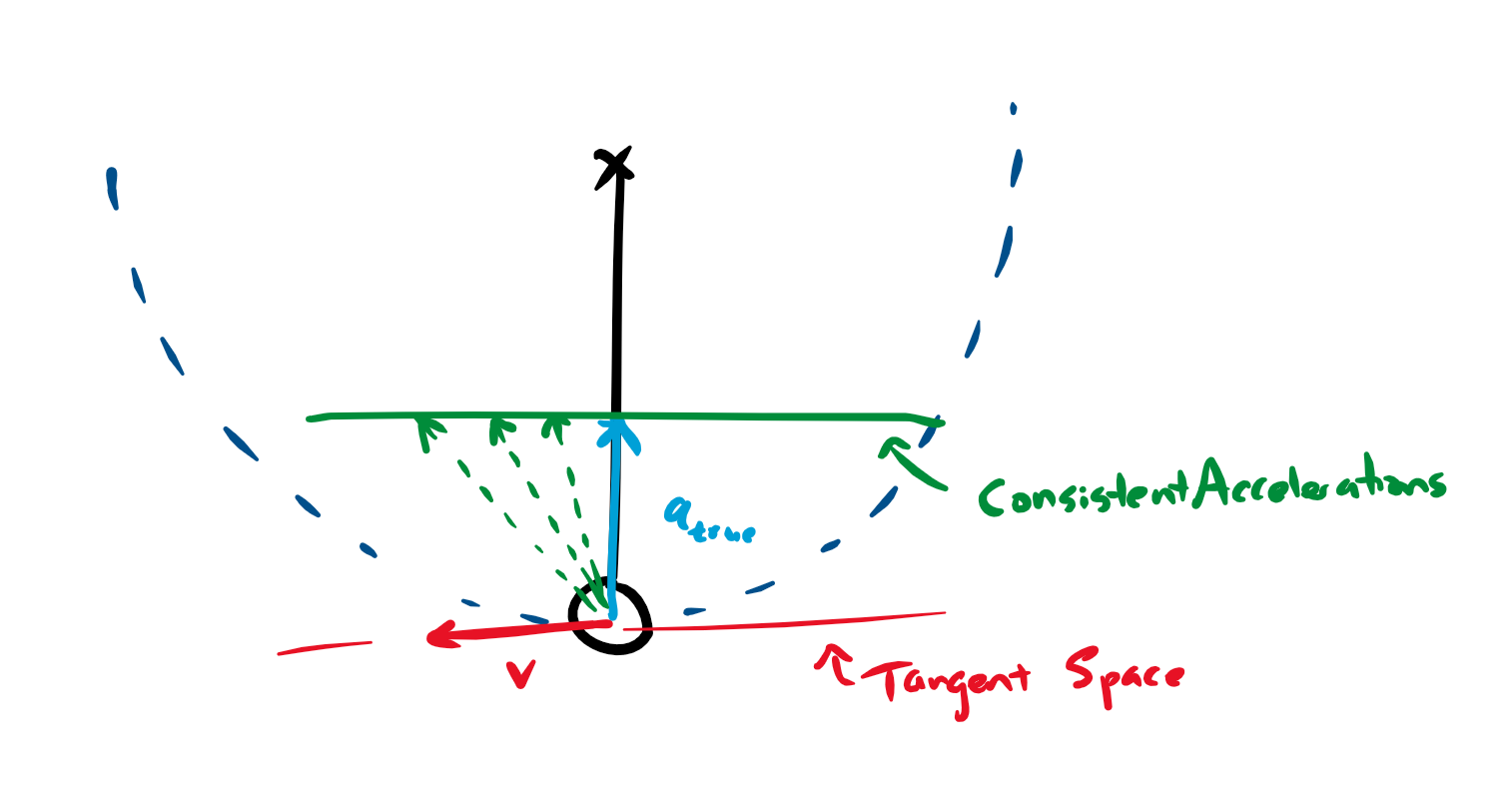The true acceleration at this point is purely radial (upwards, $a_{true}$ in blue), and the consistent accelerations (dashed green) correspond to further tangential accelerations. Note that these tangential accelerations can be identified with the tangent space of the constraint (tangential displacements).

This follows directly from differentiating the constraints. More formally: let $X_0(t)$ and $X_1(t)$ be two consistent trajectories (on the manifold), which agree in position and velocity at $t=0$. Let matrix $C_{X}$ be the (linear) constraints defining the manifold at point $X$ (ie, $C_X$ is the orthogonal complement to the tangent space $T_X$). That is, $C_{X} \dot{X_i}(t) = 0$ along the trajectory. Differentiating, \begin{align*} \frac{d}{dt}(C_{X} \dot{X_i}(t)) &= \vec 0\\ \dot{C_{X}} \dot{X_i}(t) + C_X \ddot{X_i}(t) &= \vec 0 \end{align*} Since $X_0$ and $X_1$ agree in position and velocity $(\dot{X_i)}$ at $t=0$, subtracting the last relation for the two trajectories $i=0$ and $i=1$ yields \[C_X( \ddot{X_1}(0) - \ddot{X_2}(0)) = \vec 0\] Thus, the difference in accelerations is a consistent velocity: $\ddot{X_1}(0) - \ddot{X_2}(0) \in T_X $ This shows that $\consaccel_{X, \dot X}$ is contained in an affine shift of $T_X$. (In fact, it is easy to show that this containment is an equality, but we will not need this fact).

Proof of Gauss's Princple