ENIAC: The Way We Were

When I first got interested in computers, it was all but impossible for an individual to own a computer outright. Even a “small” machine cost a fortune not to mention requiring specialized power, cooling, and maintenance. Then there started to be some rumblings of home computers (like the Mark 8 we recently saw a replica of) and the Altair 8800 burst on the scene. By today’s standards, these are hardly computers. Even an 8-bit Arduino can outperform these old machines.

As much disparity as there is between an Altair 8800 and a modern personal computer, looking even further back is fascinating. The differences between the original computers from the 1940s and anything even remotely “modern” like an Altair or a PC are astounding. If you are interested in that kind of history, you should read a paper entitled “Electronic Computing Circuits of the ENIAC” by [Arthur W. Burks].

These mid-century designers used tubes and were blazing new ground. Part of what makes the ENIAC so different is that it had a different design principle than a modern computer. It was less a general purpose stored-program computer and more of a collection of logic circuits that could be configured to solve problems — sort of a giant vacuum tube FPGA, if you will. It used some internal representations that proved to be suboptimal which also makes it seem strange. The EDSAC — a later device — was closer to what we think of as a computer. Yet the ENIAC was a major step in the direction of a practical digital computer.

Cost and Size

The size of ENIAC is hard to imagine. The device had about 18,000 tubes, 7,000 diodes, 70,000 resistors, 10,000 capacitors, and 6,000 switches. There were 5 million hand-soldered joints! ([Thomas Haigh] tells us that while this is widely reported, the real number was about 500,000.) Physically, it stood 10 feet tall, 3 feet deep, and 100 feet long. The tube filaments alone required 80 kW of power. Even the cooling system consumed 20 kW. In total, it took 150 kW to run the beast.

The cost of the machine was about $487,000. Almost a half-million dollars in 1946 is plenty. But that’s nearly seven million dollars in today’s money. What was worth that kind of expenditure? The military built firing tables for shell trajectories. From the [Burks] paper:

“A skilled computer with a desk machine can compute a 60-second trajectory in about twenty hours…”

Keep in mind that in 1946, a computer was a person. [Burks] goes on to say that a differential analyzer can do the same job in 15 minutes. ENIAC, on the other hand, could do it in 30 seconds and with a greater precision than the differential analyzer.

Keeping it Running

Tubes aren’t known for being highly reliable. In fact, an old friend of mine worked on the Whirlwind — another early computer with “only” 5,000 tubes. He said they kept good tubes in the right pocket of their lab coat and burned out tubes in the left. When the machine stopped, they would roam around looking for the dark tube and fill one pocket while emptying the other.

According to [Burks], to minimize this problem the tubes operated far below their rated values. A filament rated for 6.3V, for example, would run at 5.7V. Like a modern computer, ENIAC operated on a master clock and using digital switching to minimize timing and parameter variations in different tubes.

Cards and Decimal Delight

The original ENIAC had no memory as we think of memory. [Burks] describes that some internal memory resides in dual triodes operating as a flip-flop (also known as an Eccles-Jordan circuit). However, some function tables were no more than a matrix of resistors—this is read-only, of course. [Burks] also asserts that the plug wires also form a kind of memory. The machine did have punched card input and output and in 1953, the machine had 100 words of magnetic core added.

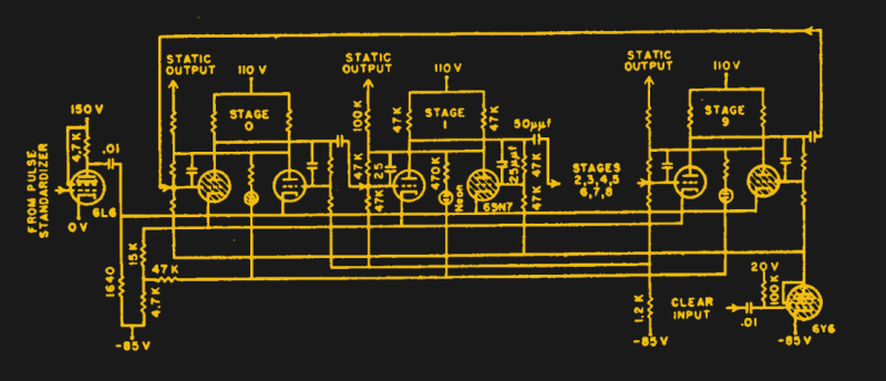
Although the machine used digital logic, it didn’t use binary. Instead, the computer used decimal digits stored in a ring counter (see schematic below). This took 36 tubes (some of which were actually two tubes in one envelope) per digit. It was the electronic analog of a mechanical counter. Pulses advance the count for each digit and an overflow advances the next virtual wheel.

Units

There were 20 ten-digit accumulators (that’s 7,200 tubes right there). These could perform 5,000 additions or subtractions per second. Some of the accumulators could multiply (385 multiplications per second) and others could do divisions and square roots. The machine could do 40 divisions per second or 3 square roots.

The speeds are somewhat misleading as it was possible to set up multiple operations to proceed at once — early parallel processing. Also, things like multiplication could go faster depending on the number of digits in the operands.

You can find a lot more detail about the device’s design in the paper. However, that’s not what you really want, is it?

Hands On

There was a time when it would have been nearly impossible to try your hand at programming the ENIAC. Now, you can simulate one using a Java program. If you decide to accept the challenge, you’ll probably want to read the operator’s manual ([Burks] was also one of the authors of the manual).

I’ll start you off with a very simple example. When you start the Applet, you can load a few example programs or some configurations. Pick the “Small” configuration which only has a few units but is easier to manage for a start. It should look like this:

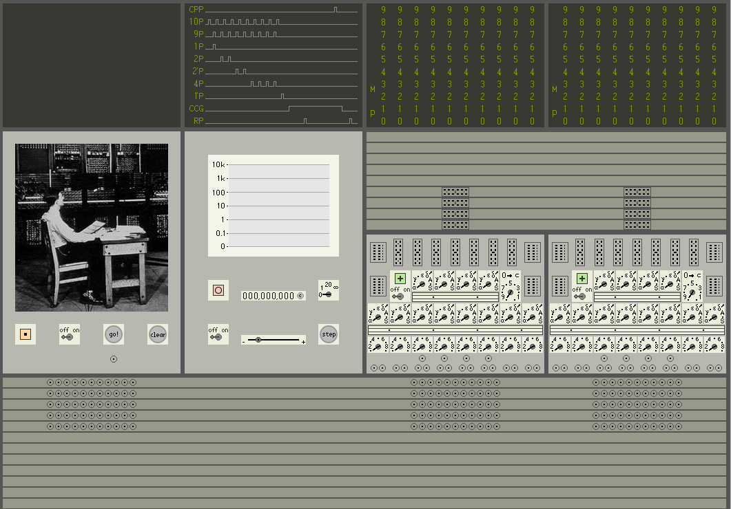
The top left box is some indicator lights (they will spell GO when running). The next box to the right shows the current clock state. The box below that controls the clock. You can set the frequency with the slider. Back to the top, the two boxes with the 0-9 lights are the accumulators. You can click on them to set a value, or just read the lights. The box with the picture in it is the initiating unit and you’ll use it to make the program run. You can let your mouse hover over the various elements to see what each part is.

The bottom rows contain interconnects. If you let the mouse float over them, you’ll see they are numbered. As you might expect, number 5 on the left connects to number 5 on the right, for example. The same arrangement is right under the accumulators, except those connect entire numbers, not just signals.

The units with all the rotary switches are where you do the bulk of the programming. If you hover your mouse over the various elements, you’ll see what each switch does (most of them are duplicates, but have different numbers; you’ll see why in a minute).

Here’s a simple setup to add six (stored in the left accumulator) into the right accumulator (use the blue numbers in the figure below if you get lost).

1. Draw a wire from the terminal on the initiating unit (the box with the picture) to the nearby program connector 1 in tray A (the leftmost terminal on the top row of the interconnect trays).
2. On the cycling unit (the clock), turn the knob to infinity.
3. In the box with the switches, there are two connectors at the left (IL1 and IL2). Draw wires between them in both boxes.
4. On the right side of tray ‘A’ there are terminals. Connect program connector 1 to program connector 1 in each accumulator box.
5. In the top right corner of each of those same boxes is a connector, IR1. Click on it to install a shorting plug (repeat for both boxes).
6. In the left box with the switches, find operation switch 1 and turn it to A (not alpha, but A).
7. In that same box, drag a cable from digit connector A to the connector in tray 1, just above it.
8. In the rightmost box with the switches, drag a cable from digit connector alpha to the nearby tray 1 connector.
9. Turn on all four filament switches (one in each unit).
10. In the left-hand accumulator, click on the 6 in the rightmost column. This represents the number 6.

After all this, your setup should look like this (except the blue numbers, of course):

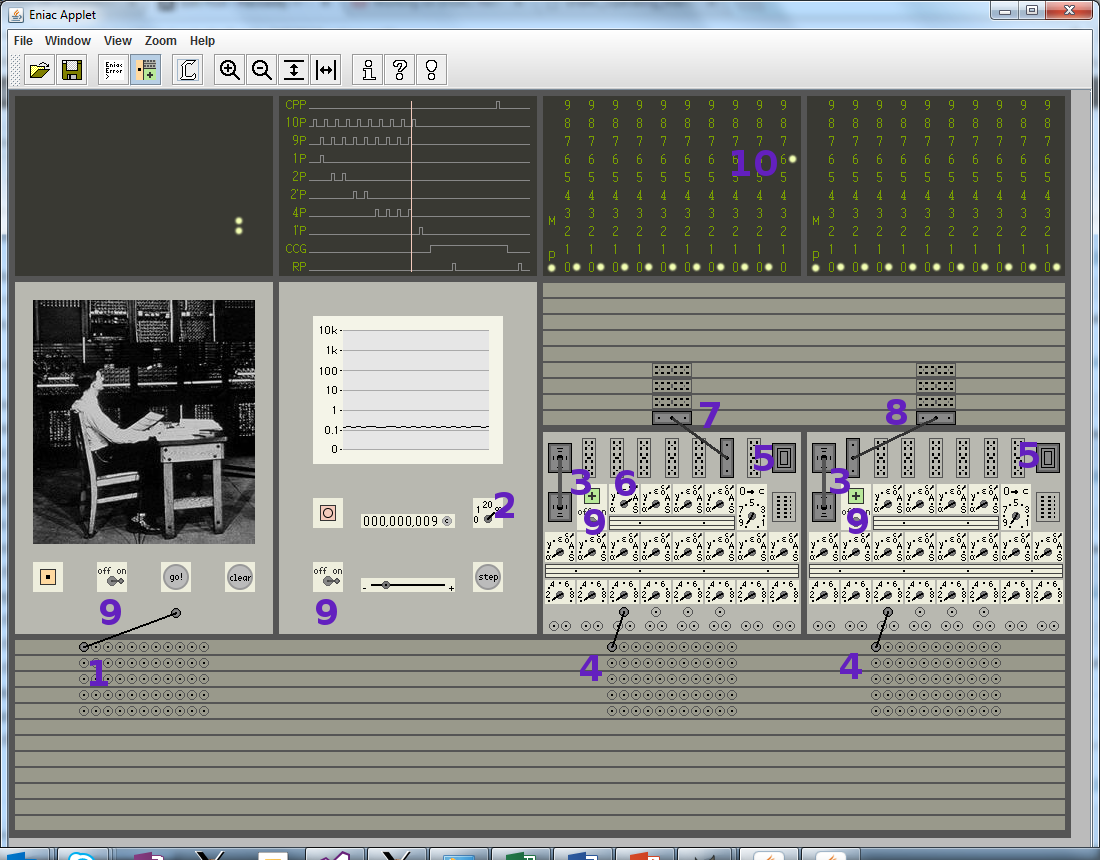
If everything looks good, press the Go button in the initiator unit. At first, it may appear that nothing is happening. If the clock is slow (which it is by default) it will take a while for things to start since the machine won’t really run until the clock starts at the beginning. This is always true, but if you crank up the clock speed, you won’t notice so much. Don’t at first, though, because it is interesting to observe the machine operate at slow speed.

You’ll see that the first accumulator actually cycles through, creating pulses to send to the other accumulator. After one cycle, it will stop and now both accumulators will contain 6. Press Go again and when things are done, the result will be 12.

Wait, What?

I told you that it doesn’t resemble modern programming very much. The short description is that the initiator causes the first accumulator to dump its contents as pulses on tray 1 (via the A output). The second accumulator receives those pulses via the alpha channel and uses them to advance the virtual wheel I mentioned earlier.

Try moving to operation 5 (instead of 1) in each accumulator. Then set repeat switch 5 to some value in both boxes (say, 4, for example). Now, the result will wind up being 6 times 4 and if you watch it execute, you’ll see why.

First Principles

Spend a day programming ENIAC and you’ll appreciate our modern tools. The emacs vs vi war doesn’t seem like such a big deal after you’ve spent a day pushing patch cords around. In general, I like the idea of going back to first principles. However, if I were teaching CPU design, I’m not sure I’d go this far back to start. Understanding how ENIAC and other computers of that period operated can give you some insights. Reading the [Burks] paper gives a lot of insight into the design tradeoffs and while the techniques aren’t likely to be useful today, the approach to solving problems can be instructive.

The Java program is neat because it runs anywhere and it is visually appealing. If you are serious about simulating the ENIAC and you don’t mind downloading some software, there are other options that simulate more of the device.

For some deep history on the construction and early use of ENIAC, you might also enjoy the video below from computer historian [Dr. Thomas Haigh]. He mentions that some of the quoted speeds for the machine were not reliable, and also points out a lot of the unsung heros behind the machine’s development. If you want to see some more example programs, you can find some on the web site for his book (look under supporting technical material).

[Featured and Thumbnail images are U.S. Army Photos via Historic Computer Images]